RNA-seq produces millions of sequences from complex RNA samples. With this powerful approach, you can:
- Measure gene expression.
- Discover and annotate complete transcripts.
- Characterize alternative splicing and polyadenylation.
The RNA-seqlopedia provides an overview of RNA-seq and of the choices necessary to carry out a successful RNA-seq experiment.
0. RNA-Seq workflow
Copy this link to clipboard
The purpose of this site is to provide a comprehensive discussion of each of the steps that are involved in performing RNA-seq, and to highlight the primary options that are available along with some guidance for choosing between various options. The primary content is topically organized according to the work-flow of a typical RNA-seq experiment.
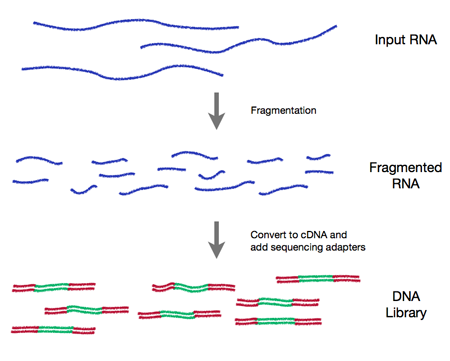
In all cases an RNA-seq experiment involves making a collection of cDNA fragments which are flanked by specific constant sequences (known as adapters) that are necessary for sequencing (see Figure 0.1). This collection (referred to as a library) is then sequenced using short-read sequencing which produces millions of short sequence reads that correspond to individual cDNA fragments.
A typical RNA-seq experiment consists of the following steps:
-
Design ExperimentSet up the experiment to address your questions.
-
RNA PreparationIsolate and purify input RNA.
-
Prepare LibrariesConvert the RNA to cDNA; add sequencing adapters.
-
SequenceSequence cDNAs using a sequencing platform.
-
AnalysisAnalyze the resulting short-read sequences.
Each of the five chapters below are dedicated to one of these steps.
Figure 0.1 RNA-Seq workflow
1. Experimental Design
Copy this link to clipboard
-
Design ExperimentSet up the experiment to address your questions.
-
RNA PreparationIsolate and purify input RNA.
-
Prepare LibrariesConvert the RNA to cDNA; add sequencing adapters.
-
SequenceSequence cDNAs using a sequencing platform.
-
AnalysisAnalyze the resulting short-read sequences.
1.1 Overview
Copy this link to clipboard
When designing an RNA-seq experiment researchers are faced with choosing between many experimental options, and decisions must be made at each step of the process. In some cases the choice one makes will have little impact on the quality of the experimental data. However, in other cases inappropriate decisions can result in spending a great deal of time and money only to obtain nearly useless data. It is therefore imperative that one carefully considers these choices before launching into a time consuming and costly RNA-seq experiment.
This stage of the experiment is arguably the most important but often receives the least amount of attention. Before one even begins an RNA-seq experiment they should have an understanding of each step and should put together a carefully devised experimental plan.
1.2 Identify the primary experimental objective.
Copy this link to clipboard
The types of information that can be gained from RNA-seq can be divided into two broad categories: qualitative and quantitative.
- Qualitative data includes identifying expressed transcripts, and identifying exon/intron boundaries, transcriptional start sites (TSS), and poly-A sites. Here, we will refer to this type of information as "annotation".
- Quantitative data includes measuring differences in expression, alternative splicing, alternative TSS, and alternative polyadenylation between two or more treatments or groups. Here we focus specifically on experiments to measure differential gene expression (DGE).
These two types of data are related and to some degree are inseparable. For instance, high quality annotation can lead to greater accuracy in mapping which can lead to higher quality measures of gene expression. Similarly, accurate annotation requires some degree of quantification. For instance, the simple existence of one or two reads that map to an intergenic region is not strong evidence for the existence of a gene at that locus.
It is important to realize that experiments that are designed to measure quantitative changes have requirements that differ from those that are designed for annotation, and it would be difficult and expensive to design a single experiment that satisfies the requirements of both. It is therefore important to first identify the primary goal of an RNA-seq experiment so that the experiment can be designed to maximize the objective. Below, we highlight some of the important distinctions between these two objectives with regards to RNA-seq. Further guidelines can be found in Table 1.1.
Table 1.1 Recommendations for RNA-seq options based upon experimental objectives.
| Criteria | Annotation | Differential Gene Expression |
| Biological replicates | Not necessary but can be useful | Essential |
| Coverage across the transcript | Important for de Novo transcript assembly and identifying transcriptional isoforms | Not as important; however the only reads that can be used are those that are uniquely mappable. |
| Depth of sequencing | High enough to maximize coverage of rare transcripts and transcriptional isoforms | High enough to infer accurrate statistics |
| Role of sequencing depth | Obtain reads that overlap along the length of the transcript | Get enough counts of each transcript such that statistical inferences can be made |
| DSN | Useful for removing abundant transcripts so that more reads come from rarer transcripts | Not recommended since it can skew counts |
| Stranded library prep | Important for de Novo transcript assembly and identifying true anti-sense trancripts | Not generally required especially if there is a reference genome |
| Long reads (>80 bp) | Important for de Novo transcript assembly and identifying transcriptional isoforms | Not generally required especially if there is a reference genome |
| Paired-end reads | Important for de Novo transcript assembly and identifying transcriptional isoforms | Not important |
1.3 Annotation
Copy this link to clipboard
The goal of annotation is to identify genes and genic architecture by analyzing short-sequence reads derived from expressed RNA. Thus, the most important parameter is that the sequence reads evenly cover each transcript, including both ends.
Coverage is primarily a function of the method used to prepare the library. Each library prep methods suffer from specific types of biases. For instance, oligo-dT priming for first-strand synthesis can be used to accurately annotate 3′-ends but often fails to evenly cover the 5′-end. Random priming suffers from uneven coverage due to sequence/structure priming biases, and can result in poor coverage of either of the ends. Some library preparation methods have been specifically designed to provide even transcript coverage, such as the SMARTer system from Clontech. Currently few publications have been devoted to evaluating the coverage and biases of different library prep methods; however, in one study (Levin et al 2010) it was observed that the dUTP-stranded method gave the best overall performance.
Regardless of the method used to prepare the libraries, each method still results in uneven coverage of individual transcripts. In order to get sequence reads that span the entire transcript more reads are required (i.e. deeper sequencing). Since the primary goal of annotation is to characterize what is present rather than how much of it is present annotation experiments can greatly benefit from enrichment procedures such as DSN normalization which reduces the proportion of reads that come from highly expressed RNAs, effectively increasing the reads that come from rarer transcripts without requiring deeper sequencing.
Two of the biggest challenges related to using short-read sequencing for annotation are that the sequence reads are much shorter than the biological transcripts and that in many cases a reference genome is unavailable. Both of these issues create problems for mapping and de novo transcript assembly. These problems can be partially alleviated by using sequencing strategies that produce longer sequence reads, paired-end reads, and stranded library preparation methods. Third generation sequencing platforms, such as PacBio, have much longer reads, which also can overcome these challenges, albeit at a greater cost than short-read sequencing.
1.4 Differential gene expression (DGE)
Copy this link to clipboard
The primary goal of DGE is to quantitatively measure differences in the levels of transcripts between two or more treatments or groups. At one level this is as simple as comparing the counts for reads that come from each transcript. However, simple read counts alone are neither sufficient for identifying differentially expressed genes nor for quantifying the degree of differences. This is largely because there is no way to know how accurately such counts reflect what was actually present in the original sample, and there is no indication of how widely expression normally varies in a given group or without treatment. Therefore in order to appropriately interpret differences in read counts one must also obtain information regarding the variances that are associated with these numbers. Several types of variances contribute to RNA-seq data including:
- Sampling variance: Even though a sequencing run is capable of producing millions of reads, these represent only a small fraction of the nucleic acid that is actually present in the library. There is therefore a built in sampling variance.
- Technical variance: Library preparation and sequencing procedures involve a series of complex chemical reactions which all contribute to between sample variance.
- Biological variance: Ultimately we are interested in measuring differences between different biological systems. Biological systems are inherently complex and very sensitive to perturbations. Thus, even in the absence of sampling and technical variance biological variance will always exist. Specifically the variance we are referring to is the nascent variance that is present within a treatment or control group.
DGE experiments must be designed to accurately measure both the counts of each transcript and the variances that are associated with those numbers. Experiments that are designed to annotate transcripts need to focus on getting even coverage across transcripts. However, in the case of DGE transcript abundance is typically measured by counting reads that map uniquely to that transcript, and even coverage along the length of the transcript is not strictly required. Similarly, long reads, paired-end reads, and stranded library preparation methods are not as important for DGE especially if a reference genome is available. Instead DGE experiments need to focus time and expense on replicates in order to obtain accurate measures of variances.
1.4.1 Replication and DGE
Copy this link to clipboard
Decisions about the number and types of replicates (individual units of statistical inference) are driven by both extrinsic and intrinsic factors. Extrinsic factors include cost, availability of samples, and feasibility of experiments. Intrinsic factors are often more difficult to grasp without prior information about the system and definitely more ambiguous from a decision standpoint. Intrinsic considerations include the degree of transcriptional variability among samples, whether certain genes or transcripts are of special interest, whether these genes of interest are expressed at low levels relative to other members of the transcriptome, and how many experimental factors are of interest (i.e. the complexity of an experimental design). Because the extrinsic considerations are often (but not always) "hard and fast", we find it useful to start from those constraints and subsequently build the study design around them. If, for example, you can really only afford to spend $X on a given experiment, it will become clear how much money you have to spend on the sequencing itself (the largest material cost). Given the sequencing throughput, you will be able to estimate how many individual samples can be sequenced at a given depth, and therefore how many replicates will be available for a range of possible experimental configurations.
1.4.2 Technical vs. Biological Replication
Copy this link to clipboard
Technical replication refers to the sequencing of multiple libraries derived from the same biological sample. Non-biological variation in estimated transcript abundance across these samples can arise from unintended differences during library preparation or sequencing. This variation is distinct from biological variation among individuals as well as variation due to the sampling process itself. One way to exploit technical variation would be to sequence a number of technical replicates from one library preparation technique and compare them statistically to additional technical replicates from another library preparation method. In this case inferences about differences in estimated transcript abundance owing to library preparation method could be drawn. In many cases, however, biologists are interested in using a single technical approach to understand biological variation among different individuals or tissues, usually with respect to experimental treatments. When biological variation is large relative to technical variation (Bullard et al. 2010) the rewards in statistical power due to additional biological replicates will surpass the improved parameterization of technical variation garnered from additional technical replicates, but technical variation does become a problem for transcripts with shallow coverage (McIntyre et al. 2011).
Unless you are genuinely interested in comparing technical aspects of RNA-seq, or you expect technical variation to be especially great for a large majority of the target transcripts, we recommend greater resource allocation to biological replication. This isn't to say technical replicates should never be sequenced, but simply that limited financial resources are probably better spent on more biological, relative to more technical, replicates in many cases.
1.4.3 How many replicates should be sequenced?
Copy this link to clipboard
As with any experiment that is intended to test a null hypothesis of no difference between or among groups of individuals, differential expression studies using RNA-seq data need to be replicated in order to estimate within- and among-group variation. We understand that constraints in some study systems make replication very difficult, but it really is important.
Statistical hypothesis tests are prone to two types of error. Failure to reject the null hypothesis of no difference when there actually is a difference (a "false negative") is known as type II error, and β is used to symbolize the probability of its occurrence. The number of replicates per group in an experiment directly affects type II error, and therefore "statistical power" (which is 1-β). Power also depends on the magnitude of the effect of one condition relative to another on the variable of interest, which is in part determined by the degree of variation among individuals. Thirdly, power depends on the acceptable maximum probability of type I error (the event in which the null hypothesis is rejected in favor of the alternative when the null hypothesis is actually true). Experimenters conventionally tolerate the risk of type I error (symbolized by α) if it is less than 0.05 for a given test. When performing many hypothesis tests (as is the case for differential expression tests across thousands of transcripts), type I error must be considered in light of the many tests. For example, if one performs 20,000 tests of differential expression with an "acceptable" type I error probability of < 0.05, 1,000 rejections ofnull hypotheses are expected due to chance alone. So if you identify 2,000 differentially expressed genes under this scenario, half of these are likely false positives! Given this problem it is common practice to instead identify a group of genes for which the expected "false discovery rate" is a sufficiently low value (e.g. 0.1), given the distribution of p-values across all of the many hypothesis tests. For a more detailed description of multiple hypothesis testing for highly dimensional data, we recommend an excellent review (Noble 2009). For statistical approaches commonly used to control the false discovery rate in genomic data sets, see (Benjamini, Hochberg 1995) and (Storey 2002).
In order to estimate how many replicates to sequence for a given hypothesis test to achieve a desired level of power, you need to have at least a crude handle on treatment effect size, which depends on variance in read counts across individuals within each treatment. Note that effect sizes are easier to reliably estimate for genes with at least moderate sequencing coverage in one treatment than for genes with sparse coverage in all treatments (e.g. < 10 reads per individual), so sequencing depth for each transcript needs to be considered. Finally, because power is also a function of α, it is useful to have an estimate of the acceptable p-value threshold which has been adjusted, of course, to reflect an acceptable false discovery rate. This parameter depends on the number hypothesis tests and the distribution of original p-values across those tests.
While it is impossible for anyone to say with complete accuracy how many replicates are necessary for any given experimental objective, there are a few key guidelines relevant to the issues described above that will at least help you avoid conducting a completely ineffective study. The major considerations that dictate these guidelines are listed below. Additional relevant information may be found in the Analysis section in this website.
1.4.4 Depth of Sequencing
Copy this link to clipboard
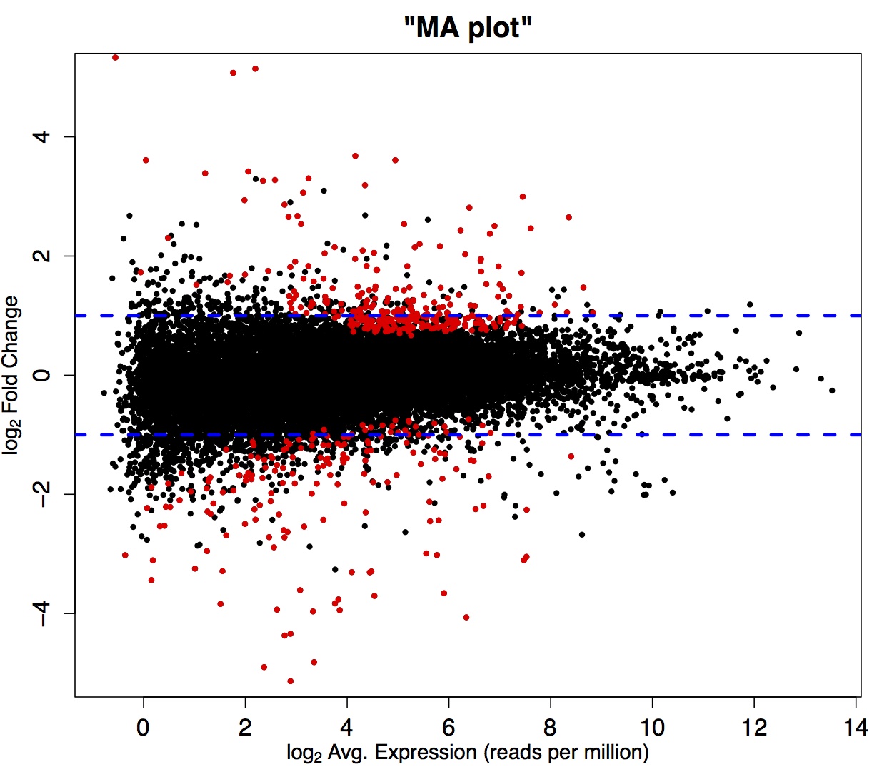
As mentioned previously, variation due to the sampling process makes an especially large contribution to the total variance among individuals for transcripts represented by few reads. This means that identifying a treatment effect on genes with shallow coverage is not likely amidst the high sampling noise (see Figure 1.1).
A study of chicken RNA-seq data revealed that expression estimate correspondence among technical replicates (no biological variation) for genes with above-median coverage stabilized at about 10 million reads per sample (Wang et al. 2011). It therefore stands to reason that 10 million reads per sample is a benchmark from which to start, although this is by no means a hard and fast rule for all data set types.
Figure 1.1
1.4.5 Experimental Complexity
Copy this link to clipboard
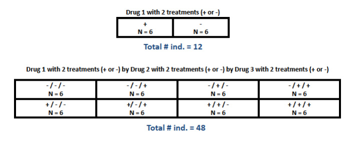
A comparison between two groups (e.g. one "experimental" and one "control") is the simplest type of differential expression study design, and probably a fairly common one. For more complex designs, however, it is important to remember that sufficient replication has to occur at every level of comparison. In a fully "factorial" design, for example, more than one experimental "factor" is of interest, each with two or more treatments, such that any individual receives one of multiple possible treatments at each factor. In this case, every possible combination of treatments across factors needs to be replicated sufficiently, which results in a much larger total sample size (see Figure 1.2). Many more complicated design classes are possible. A formal, comprehensive treatment of experimental design is beyond the scope of this website, so please consult an appropriate biometry text, Sokal and Rohlf's Biometry is one very suitable reference.
Figure 1.2
1.4.6 Target Transcript Properties
Copy this link to clipboard
The nature of the individual transcripts in which one is most interested will undoubtedly dictate the success of an RNA-seq study. For instance, if you have no expectations for differential expression and simply want a preliminary list of candidates that are grossly differentially expressed, you are likely to reach this goal. If, on the other hand, you are interested in testing whether very specific sets of transcripts are different in abundance among treatments, and you have reason to believe they might be expressed at low levels, you may not reach sufficient coverage (even with tens of millions of reads per sample) to detect a real difference. In general, detecting all real differences in expression across the entire transcriptome is not a realistic expectation given the statistical issues addressed above.
1.4.7 Treatment Effect Size
Copy this link to clipboard
As mentioned above, the effect size will to some extent be affected by sampling variance, and therefore by depth of coverage. There are also clear biological reasons to expect differences in effect size across transcripts or specific types of samples. Some treatments will simply affect transcriptional targets more directly than others, so large differences between treatments for these targets are expected. Some transcriptional responses to a treatment may be more variable among individuals, owing to greater genetic variation at the regions of the genome responsible for mediating the response, which will ultimately manifest as a smaller effect size. In some cases very large, extensive transcriptional differences are expected across the board. If, for example, one is comparing transcript abundance between two different tissue types, many large differences at the level of read counts are expected.
1.5 No Substitute for "Pilot" Data
Copy this link to clipboard
You have probably noticed that these key considerations (especially target transcript attributes and effect sizes) seem likely to vary widely on a case-by-case basis. Factors like the nature of the treatment(s), the type of sample, or the ability to control the environment of subjects, for example, really differ from experiment to experiment. This means that published data from some other experimental system, or even naïvely simulated data, may not be informative enough for critical decisions up front. In light of this conundrum, our single best recommendation is to first sequence a subset of replicates from a larger experiment, get a handle on coverage levels across genes and effect sizes of treatments, and then use this information to estimate the level of replication necessary to reach a given level of statistical power for a given fraction of the transcriptome. One strategy, provided the experimental setup is not too costly, might be to run the desired experiment with a substantial level of replication (e.g. 10-20 individuals per treatment or combination of treatments), but only actually sequence 3 or 4 samples at moderate to high coverage (e.g. 10 million reads per individual) for each treatment level. This way you would have enough preliminary information to conduct a reliable power analysis, but still have plenty of remaining samples "in the bank" for additional sequencing.
Fortunately, the Marth Lab at Boston College has produced a handy, flexible tool for estimating power of RNA-seq study designs, given a suite of user-supplied parameters. This tool, called "Scotty" (Busby et al. 2013), is especially effective when fed user-supplied pilot data, and will output a range of sample size/coverage configurations acceptable for specified power and cost constraints. The tool may be found here. Although this tool is currently designed to accommodate a simple two-treatment experimental design, the framework is in principle extendable to more complicated designs.
2. RNA Preparation
Copy this link to clipboard
-
Design ExperimentSet up the experiment to address your questions.
-
RNA PreparationIsolate and purify input RNA.
-
Prepare LibrariesConvert the RNA to cDNA; add sequencing adapters.
-
SequenceSequence cDNAs using a sequencing platform.
-
AnalysisAnalyze the resulting short-read sequences.
2.1 Overview
Copy this link to clipboard
Since the goal of RNA-seq is to characterize the transcriptome the first step naturally involves isolating and purifying cellular RNAs. Isolation and purification of RNA typically involves disrupting cells in the presence of detergents and chaotropic agents. Depending upon the starting material mechanical disruption is also recommended. After homogenization, RNA can be recovered and purified from the total cell lysate using either liquid-liquid partitioning or solid-phase extraction. Typically the total RNA is then enriched for messenger RNA (mRNA). This can be done by either directly selecting mRNA or by selectively removing ribosomal RNA (rRNA). To make the RNA suitable for RNA-seq it is typically fragmented and then the quality and fragmentation are assessed.
2.2 Working with RNA
Copy this link to clipboard
The success of RNA-seq experiments is highly dependent upon recovering pure and intact RNA. Because RNA is more labile than DNA and RNases are very stable enzymes extra care should be taken when purifying and working with RNA. Some general considerations are:
Precautions when working with RNA
- Maintain separate reagents and consumables for RNA extraction. Avoid co-storage with reagent kits that include RNases.
- Process the samples quickly and keep the RNA on ice when possible.
- Wear gloves and work in a clean workspace.
- Use RNase free water. Water from commercial purifiers is generally RNase-free (as long as the purifier and dispensers are kept thoroughly clean). To ensure that water is RNase-free it can be treated with diethyl pyrocarbonate (DEPC) as follows. Add DEPC to 0.05% and incubate overnight at room temperature. The DEPC is then destroyed by autoclaving for 30 minutes.
- Glassware can be heated at 250 °C for several hours to remove RNase contamination.
- Plastic-ware can be soaked in 0.1 N NaOH/1mM EDTA then rinsed thoroughly with RNase free water.
Other information about working with RNA can be found at: Working with RNA (Ambion).
2.3 Stabilize RNA
Copy this link to clipboard
The overall goal of RNA-seq is to characterize the transcriptome at the moment the cells were harvested; thus care should be taken to limit degradation of RNAs.
More on RNA stabilization
More on RNA stabilization
RNA is much more labile than DNA, and the moment a tissue sample is dissected, for example, the cells begin to die and the RNA begins to be degraded. Since there is often a time delay between harvesting and isolation of the RNA samples should be frozen in liquid nitrogen immediately upon harvest. In addition several reagents have been developed to preserve the RNA in fresh tissue. Two of the more commonly used reagents are RNAstable® (from Biomatrica) and RNAlater® (from Qiagen). Carefully follow instructions in the manuals for stabilization reagents. Qiagen also sells a reagent (RNAprotect Bacteria Reagent) that is specifically formulated for bacteria. Even if the samples can be frozen immediately it is recommended that an RNA stabilizer is added before freezing since the moment the tissues begin to thaw in the subsequent extraction the RNAs are subject to degradation.
2.4 Isolate and purify RNA
Copy this link to clipboard
Two of the primary challenges of the isolation procedure are (1) to separate the RNA from other cellular materials and (2) to preserve the integrity of the RNA that is extracted. This is complicated by the fact that DNA and RNA are chemically very similar to each other and that RNases are notoriously stable proteins that can still be active under conditions that denature other proteins.
2.4.1 Solubilization
Copy this link to clipboard
Virtually all RNA extraction procedures rely upon disrupting tissues in an aqueous solution containing organic buffers, guanidinium salts, and ionic detergents.
More about RNA solubilization
More about RNA solubilization
The buffers that are most commonly used include TRIS and sodium-acetate, which are added to adjust and maintain the pH. Chaotropic agents (compounds that disrupt both hydrophobic and hydrogen-bond interactions) are added to denature proteins. The most commonly used chaotropic agents are guanidinium salts. Guanidinium is a strong protein denaturant capable of denaturing recalcitrant proteins such as RNases. The benefits of using guanidinium for purification of RNA were first reported in 1951 (Volkin and Carter 1951) and since that time virtually all RNA extraction procedures have incorporated the use of high concentrations (4-6M) of guanidinium thiocyanate or guanidinium hydrochloride. Ionic detergents are added to help solubilize cell membranes and lipids. The most commonly used detergents include sodium dodecyl sulfate (SDS), sodium lauroyl sarcosinate (sarkosyl), sodium deoxycholate, and cetyltrimethylammonium bromide (CTAB).
2.4.2 Mechanical Homogenization
Copy this link to clipboard
Incomplete homogenization can significantly reduce RNA yields.
Different types of samples require different methods to completely disrupt cells.
More about tissue homogenization
More about tissue homogenization
Despite the presence of detergent and chaotropic agents it is necessary to also incorporate some form of mechanical homogenization to completely disrupt cell walls, plasma membranes, and organelles. For some samples, such as mammalian cell cultures, addition of chaotropic agents is enough to lyse the cells. However, mechanical homogenization is still recommended to shear the DNA and assist in the solubilization of organelles. For cell cultures the homogenization can be as simple as rapidly pipetting the sample or passing it through a syringe needle several times. Other tissues require more extreme mechanical processing.
Mechanical methods for homogenizing tissues include using cryo-grinding with a mortar/pestle, shearing using a rotor-stator homogenizer or a Dounce homogenizer, sonication, or bead-beating. The method that one should choose is highly dependent upon the starting material. The following links provide useful information for choosing appropriate homogenizers.
Tissue specific considerations
Isolation of RNA from muscle and skin tissues can be difficult due to the presence of connective tissue, collagen, and contractile proteins. For these tissues proteinase K can be added to degrade the problematic proteins. Proteinase K is an especially robust enzyme that retains activity under conditions that denature most other proteins. For these samples it is generally advised to first use mechanical homogenization in high concentrations of guanidinium. Then the homogenate should be diluted to decrease the guanidinium concentrations to ~2M before adding the proteinase K. However, researchers should be aware this dilution step can affect the downstream purification and in all cases they should follow protocols that have been developed specifically for these tissues.
Tissues high in fat:Homogenates from tissues that are high in fat (e.g., brain, adipose tissue, and plant seeds) should be extracted with chloroform to remove lipids.
2.4.3 Recovery of RNA from lysate
Copy this link to clipboard
After homogenization two methods are commonly used to recover RNA from the cell lysate. (1) by extraction with organic solvents or (2) by solid-phase extraction on silica.
2.4.3.1 Organic extraction
Copy this link to clipboard
One of the oldest methods for recovering RNA from the lysate involves using a mixture of acidified phenol/chloroform/isoamyl alcohol.
More on organic extraction
More on organic extraction
Use of phenol for recovering RNA was first reported in 1956 (Kirby 1956), and in 1987 Chomczynski and Sacchi presented the method that is still used today (Chomczynski and Sacchi 1987; Chomczynski and Sacchi 2006). Acidified phenol/chloroform/isoamyl alcohol is added to the cellular homogenate, mixed to make an emulsion and then the organic and aqueous phases are separated by centrifugation. Generally a third phase (the interphase) also forms between the lower organic and upper aqueous phases. The aqueous phase contains the RNA while denatured proteins and lipids preferentially partition into the interphase and organic phase. The aqueous phase can be recovered by pipet. Under acidic conditions (pH ~4.8) DNA preferentially partitions into the organic phase. It is important to realize that the pH is a critical factor in this technique since at higher pH DNA will end up in the aqueous layer and contaminate the RNA.
Many researchers choose to use one of several premixed solvents that are based on the Chomczynski protocol. Some of the commonly used products include: TRIzol (Life Technologies), TRIsure (Bioline), and PureZOL (BIO-RAD).
After pipetting off the aqueous layer the RNA is typically concentrated and desalted using ethanol or isopropanol precipitation.
Considerations when using phenol/chloroform partitioning
- One of the most common mistakes is to start with too much tissue, since the pH, and the concentrations of guanidinium, phenol, and chloroform are all critical factors.
- Care must be taken to ensure that none of the interphase or organic phase is withdrawn during removal of the aqueous layer. It is better to sacrifice some of the aqueous layer than to try to recover all of it. If it is very important to recover all of the RNA then it is better to recover a safe amount of the initial aqueous layer then add more extraction buffer and perform a second extraction. The two aqueous layers can then be combined and ethanol precipitated.
- After the phenol/chloroform extraction it is often beneficial to perform a final extraction using just chloroform to remove traces of phenol, which can inhibit downstream reactions.
2.4.3.2 Solid-phase extraction
Copy this link to clipboard
An alternate procedure for separating RNA from other cellular macromolecules involves using solid-phase extraction onto silica. The RNA is bound onto the surface of silica fibers directly out of cellular lysate, washed of contaminants while bound, and then eluted back into solution.
More on solid-phase extraction
More on solid-phase extraction
In the 1970's it was demonstrated that nucleic acids in the presence of high concentrations of chaotropic agents would bind to silica. Since nucleic acids and silica are both negatively charged the interaction is not simply due to charge-charge interactions. Instead, binding is thought to be due to the formation of a cationic salt bridge, which is promoted by chaotropic compounds. This phenomenon formed the basis of procedures designed to recover and purify nucleic acids from cell lysates.
When using this technique to purify RNA the guanidinium serves to both denature proteins and promote binding to the silica. Tissues are homogenized in the presence of guanidinium first then alcohol (typically ethanol or isopropanol) is added before the lysate is applied to a small column containing silica. It is important to realize that the final concentrations of guanidinium and alcohol are crucial for success and in all cases researchers should carefully follow established protocols. Centrifugation or a vacuum is then used to force the lysate through the column after which it is washed using salt solutions that do not disrupt the nucleic acid: silica interaction but remove proteins and other cellular debris. After washing, the nucleic acid is eluted from the column using a low ionic strength buffer. Since the bound RNA can be eluted using very small amounts of elution buffer, concentration by ethanol precipitation is not generally needed before proceeding to downstream procedures. Before the advent of commercially available kits researchers built their own columns using diatoms or crushed glass. However, numerous kits are now commercially available and these are now the method of choice. Several of the most commonly used kits are available from Qiagen, Promega, Agilent Technologies, and Ambion|Life Technologies.
Solid-phase extraction vs. organic extraction
Both techniques are commonly used. However each has certain advantages and disadvantages. If appropriate care is taken both techniques are capable of producing highly purified RNA.
- Organic extraction is cheaper and is easier to scale up for larger amounts of starting material.
- Silica columns are more expensive but are easier to use and are more amenable for processing multiple samples in parallel.
- Solid-phase extraction has the advantage that the RNA can be eluted using very small amounts of elution buffer, which obviates the need to perform an ethanol precipitation step.
In practice many protocols actually combine both procedures. In this case, after adding appropriate amounts of alcohol to the aqueous phase from the phenol/chloroform extraction, it is further purified using a silica column.
Small RNAs
It should be noted that protocols for isolating mRNA are not generally optimized for isolating small RNAs such as siRNA, piwiRNA, and miRNAs. If the researcher is interested in purifying these RNAs then they must be sure to use methods that have been specifically designed for small RNAs.
Removing genomic DNA contaminants
Generally, if one carefully follows established protocols very little genomic DNA is carried over into the final total RNA sample. However, it is sometimes necessary to digest DNA using DNase I.
Another useful online guideline for RNA preparation from Ambion can be found here.
2.4.4 Quantitation and Quality Assessment
Copy this link to clipboard
The purity and/or yield of the RNA can be measured using a spectrophotometer, fluorometer or Bioanalyzer/Fragment Analyzer. And the quality of a total RNA prep can be assessed for signs of degradation by running a portion on an agarose or acrylamide gel or by using an instrument such as the Agilent Bioanalyzer.
2.4.4.1 Assessing RNA quality
Copy this link to clipboard
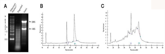
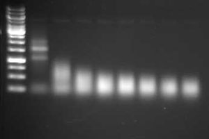
Agarose and acrylamide gels are commonly used, since most labs have the necessary equipment; however, compared to the Bioanalyzer relatively large amounts of RNA are required. Examples of good and poor quality RNA preps are shown in Figure 2.1A (agarose gel) and Figure 2.1B, 2.1C (Bioanalyzer trace).
Figure 2.1 Intact vs. degraded RNA.
2.4.4.2 Assessing RNA quantity
Copy this link to clipboard
The most commonly used methods for assessing the quantity of RNA include using: UV absorbance, fluorescence, and an Agilent Bioanalyzer. Each of these methods has strengths and weaknesses. We recommend fluorometry for quantification and the Bioanalyzer (or equivalent device) for quantification and RNA integrity evaluation. For a useful (albeit slightly dated) comparison of methods see Aranda et al. 2009.
A fluorometer (such as Life Technologies' Qubit) measures the concentration of RNA bound to a fluorescent dye. The method is not as subject to skewing by contaminants such salts, detergents, etc, as UV absorbance.
The concentration of RNA can also be estimated from a Bioanalyzer or Fragment Analyzer trace using the proprietary software. The accuracy of this method may be the least sensitive to contaminants such as DNA and phenol.
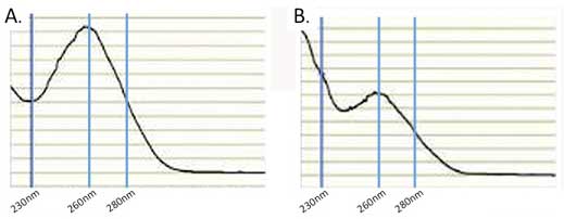
The oldest and perhaps most common way to quantitate RNA is by measuring the absorbance at 260 nm.
More on quantitation by UV absorbance
More on quantitation by UV absorbance
A 40 µg/ml solution of RNA in a cuvette with a 1 cm path length has an A260 = 1.0. To ensure an accurate reading the absorbance should be between 0.1 and 1.0.
Large errors in the quantitation can be introduced by the presence of interfering compounds that also absorb at 260 nm. To help guard against this problem it is important to examine the absorbance profile from 220-300 nm. The profile should look similar to that in Figure 2.1A which is typical for clean nucleic acid.
If the profile looks nothing like this then there is a problem. Either there is no RNA or the RNA is contaminated with other UV absorbing compounds. Some of the most common contaminants that can interfere include DNA, phenol, guanidinium, and protein all of which also absorb at 260 nm. In addition RNA isolated from plants is often contaminated with compounds such as polysaccharides, flavones, and polyphenols, all of which can lead to erroneous absorbance measurements. A common recommendation is to evaluate the A260/A280 ratio. Pure RNA has an A260/A280 ratio of 2. If there is significant protein contamination this ratio will be less than 2. However, this method alone will not accurately catch guanidinium and phenol contamination. Both of these compounds strongly absorb at 230 nm so the A260/A230 ratio can be used to determine if they are present (see Figure 2.1B). Pure RNA as an A260/A230 ratio of 2 and a value less than this is a good indication that there are contaminants. Typically, UV absorbing contaminants can be removed by either cleaning the RNA on a silica spin-column or by using ethanol precipitation.
Absorbance measurements should always be made on RNA that is suspended in a buffered aqueous solution like TE buffer (10 mM TRIS, pH 8, 1 mM EDTA). The UV absorbance of RNA is not pH dependent but that of many common contaminants is. TE has little absorbance from 230-280 nm so it will not interfere with the assay; however it is always a good practice to blank the spectrophotometer with the RNA resuspension buffer.
Figure 2.2
2.5 Target enrichment
Copy this link to clipboard
It is often necessary to enrich specific classes of RNA in the sample to be sequenced. Total RNA recovered using the procedures described above consists of >80% ribosomal RNA (rRNA) (Raz et al. 2011), so if rRNA were not removed, the majority of the final sequence reads would be from rRNA.
The four methods that are commonly used to enrich specific classes of RNAs are:
- Selection of target RNAs via hybridization.
- Removal of non-target RNAs via hybridization.
- Copy-number normalization via duplex-specific nuclease digestion.
- Target enrichment via size-selection
2.5.1 Selection of mRNAs via hybridization to oligo-dT
Copy this link to clipboard
2.5.1.1 Fishing out mature mRNA by the tail
Copy this link to clipboard
This method uses oligo-dT to selectively recover mature mRNAs by duplexing with their poly-A tails. At the same time, the proportions of RNA classes that don't have long poly-A stretches will be reduced.
More about selection of mRNAs via oligo-dT hybridization
More about selection of mRNAs via oligo-dT hybridization
Several variants of this method have been developed; these include using columns containing oligo-dT bound to cellulose, using oligo-dT bound to plastic plates via a biotin linkage, and using magnetic beads to which oligo-dT has been attached via a biotin linkage. All of these approaches work well and numerous commercial kits are available.
Since this method only recovers poly-adenylated RNAs it is useful for characterizing the levels of mature mRNAs, but other RNAs such as immature mRNAs and poly-A- non-coding RNAs (ncRNAs) will be lost.
Some mitochondrial mRNAs are also poly-adenylated and will be enriched by oligo-dT.
Bacterial mRNAs are not poly-adenylated, and therefore cannot be enriched using oligo-dT based hybridization methods.
2.5.1.2 SuperSAGE enrichment for 3′ mRNA tags
Copy this link to clipboard
SuperSAGE, a high-throughput version of SAGE (serial analysis of gene expression), is an approach that targets for sequencing just the 3′-end of transcripts with a polyA tail. SuperSAGE is especially powerful for differential gene expression because sequencing coverage is focused on a short, 3′ region of each transcript and not lost on other regions. The limitation is that one needs a well-annotated genome or transcriptome against which to align the tags, which predominantly fall in 3′ UTRs. Furthermore, this approach does not capture alternative splicing effectively.
More on SuperSAGE
More on SuperSAGE
Biotinylated oligo-dTs that include an EcoP15I recognition site are hybridized to polyadenylated mRNAs in the sample, followed by first- and second-strand cDNA synthesis. The cDNA is then cut upstream of the polyA tail with a frequent-cutting restriction enzyme such as NlaIII, and pulled down with streptavidin-coated beads. At this point an adapter, which includes the platform-specific nucleotides necessary for high-throughput sequencing, another EcoP15I recognition site, and a NlaIII overhang is ligated to the bead-bound tags. EcoP15I digestion will then cut the cDNA at a distance 25-27 nt from the recognition sequence, and this portion of the tag is sequenced after ligation of another adapter with platform-specific nucleotides, and PCR amplification.
A recent review of the technique and platform-specific protocols are described in Matsumura et al. 2012.
2.5.2 Removal of ribosomal sequences via hybridization
Copy this link to clipboard
Several companies provide kits that can be used to selectively remove ribosomal RNA from total RNA samples. In contrast to polyA+ enrichment, this approach preserves non-polyadenylated RNAs allowing one to investigate broader classes of RNAs including immature mRNAs and non-polyadenylated ncRNAs.
This technique uses oligos that are complementary to highly conserved ribosomal RNA sequences to bind and remove the rRNA.
More on rRNA depletion by hybridization
More on rRNA depletion by hybridization
The oligo/rRNA complex is removed from the solution via binding to beads. Different kits use different technologies to capture the bound complex. The capture oligos in the Ribominus (Invitrogen/Life Technologies) and Ribo-Zero (Epicentre/Illumina) kits have a biotin tag, that can be captured using streptavidin coated magnetic beads. The GeneRead kit (Qiagen) uses antibodies that specifically recognize the rRNA/oligo complex.
All of these kits are capable of removing the majority of rRNA from a total RNA sample. However, users that are working with non-model organisms should consult the manufacturer to verify that the capture oligos are compatible with the rRNA in their sample. In addition, since these kits rely upon a limited number of oligos they only work well if the input RNA is not degraded. It is therefore important that users verify the quality of their RNA before proceeding.
The mRNA-ONLY kit (Epicentre/Illumina) uses a 5′-phosphate dependent exonuclease to degrade RNAs (such as rRNA) that have a 5′-monophosphate. This exonuclease will not degrade intact and mature mRNAs that have a 5′-cap. However, the manufacturer does not recommend this kit for RNA-seq.
2.5.3 Copy-number normalization via duplex-specific nuclease digestion (DSN)
Copy this link to clipboard
The concentration of specific mRNAs varies dramatically within a cell. Some transcripts may be present at relatively high concentrations (>10,000 copies per cell) while for others there may be only a few copies. Therefore much deeper sequencing is required to interrogate the low abundance transcripts. DSN-normalization is a technique that partially normalizes the concentrations of each mRNA by selectively removing many of the most abundant transcripts, which effectively increases the relative concentration of the low abundance transcripts (Zhulidov 2004 and Zhulidov 2005). DSN can therefore be very useful for RNA-seq experiments that have annotative goals such as gene-discovery and characterization of transcript architectures (see for instance Ekblom et al. 2012).
More on DSN normalization
More on DSN normalization
DSN-normalization is performed after preparation of cDNAs and prior to library cloning. After denaturation of ds cDNA flanked with known adapters, it is subjected to renaturation. During renaturation, abundant transcripts re-anneal more quickly than those that are less abundant. Two fractions are formed: a double-strand fraction of abundant cDNA and a normalized fraction composed of single-stranded cDNA. The double-stranded cDNA fraction is then degraded by a duplex-specific nuclease (DSN).
For additional information regarding DSN see also: evrogen and sequensys.
2.5.4 Target enrichment via size-selection
Copy this link to clipboard
This method is generally reserved for enrichment of small ncRNAs such as miRNA, siRNA, and piRNAs. Since these RNAs are much smaller than mRNA and rRNA they can be separated by electrophoresis of the total RNA through an agarose or acrylamide gel and then by cutting out the region that corresponds to the size of interest. Although effective, this method is laborious and recoveries can be low. Several companies now offer small RNA purification kits that are based on solid phase extraction.
2.6 RNA fragmentation
Copy this link to clipboard
Most current sequencing platforms are capable of providing only relatively short sequence reads (~40-400bp depending upon the platform). Therefore, most protocols incorporate a fragmentation step to improve sequence coverage over the transcriptome. However, protocols differ as to when the fragmentation is performed. Most of the original protocols fragmented cDNA; however, fragmentation of the RNA (before converting it to cDNA) is becoming more popular. Four different methods are commonly used to fragment RNA: enzymatic, metal ion, heat, and sonication.
Although all of these methods are commonly used to fragment RNA, little information has been published comparing their relative performance. The goal is to produce a population of RNA fragments that are on average about 200 bp. The effectiveness of the fragmentation reaction should be assessed by evaluating the RNA on a gel or by using an Agilent Bioanalyzer. An example of fragmented RNA can be seen in Figure 2.3. This example and guidelines for fragmenting RNA can be found at the U. of Texas at Austin FGRS site.
More on mechanisms of fragmentation
More on mechanisms of fragmentation
Enzymatic
Enzymatic fragmentation is generally performed using E. coli RNase III. RNase III randomly cleaves double-stranded portions of RNA and leaves a 5′-phosphate and a 3′-hydroxyl.
Metal ionChemically induced fragmentation uses metal ions that act as Brönsted bases to abstract a proton from the 2′-OH groups of the riboses (Forconi and Herschlag 2009). This generates a 2′-O- group that attacks the phosphorous atom, resulting in departure of the 5′-OH group. This reaction results in 5′-OH and 3′-phosphates. The kinetics for this reaction are much faster for single-stranded regions of RNA. Most metal ions are capable of fragmenting RNA with differing levels of efficiency. Lanthanide ions (e.g. Eu3+, Tb3+, and Yb3+) are particularly efficient. However, the ions that are most commonly used are Zn2+ and Mg2+. Fragmentation is performed at high temperatures (70-90 °C) and slightly alkaline pH (pH 8-9). The reaction can be easily stopped by the addition of a metal chelator such as EDTA.
HeatRNA can also be fragmented by heating at 95 °C in water for 30 minutes.
SonicationRNA can be fragmented using sonication. Sonication uses high intensity sound waves to produce micro-bubbles that upon collapse release large amounts of energy capable of breaking ribonucleic-acid bonds.
Figure 2.3
3. Library Preparation
Copy this link to clipboard
-
Design ExperimentSet up the experiment to address your questions.
-
RNA PreparationIsolate and purify input RNA.
-
Prepare LibrariesConvert the RNA to cDNA; add sequencing adapters.
-
SequenceSequence cDNAs using a sequencing platform.
-
AnalysisAnalyze the resulting short-read sequences.
3.1 Overview
Copy this link to clipboard
After obtaining an RNA preparation that is suitable for RNA-seq the RNA must be converted to double-stranded complementary DNA (cDNA). Currently available sequencing technologies require a DNA template with platform-specific "adaptor" sequences at either end of each molecule. Generating the cDNA, adding the adaptors, and amplifying the DNA for sequencing round out the process of "library preparation". Competing RNA-seq procedures diverge during library preparation, and the protocol details are highly dependent upon which strategy and sequencing platform is used.
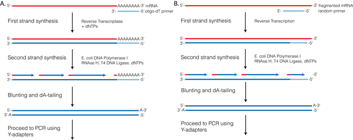
3.2 First-strand synthesis
Copy this link to clipboard
In order to convert RNA to DNA the RNA must be used as a template for DNA polymerase. Most DNA polymerases cannot use RNA as a template. However, retroviruses encode a unique type of polymerase known as reverse transcriptases, which are able to synthesize DNA using an RNA template.
All of the current protocols utilize the ability of reverse transcriptase (RT) to synthesize a DNA strand using RNA as a template. RT, like other polymerases, requires a primer annealed to either DNA or RNA to initiate polymerization. Several first-strand priming options are used. These include the following:
- Using oligo-dT to prime off of the poly-A tail of mature mRNA.
- Using random primers to prime at 'random' positions along the RNA molecule.
- Priming off of oligos that are ligated onto the ends of the RNA.
Each of these priming options has strengths and weaknesses which are discussed more fully below.
More on first-strand synthesis
More on first-strand synthesis
RTs, like other polymerases, can only initiate synthesis from a primer with a 3′-OH that is annealed to the template strand. Several first-strand priming options are used for RNA-seq. Priming options can be divided into two major categories (1) priming off of an oligo ligated to the 3′-end of the RNA template, or (2) using primers with random sequences that can direct synthesis at random locations throughout the RNA template. The most commonly used priming methods are discussed more fully below.
Figure 3.1
3.2.1 First-strand priming using oligo-dT
Copy this link to clipboard
One of the oldest methods for first-strand priming involves using oligo-dT to prime synthesis off of the poly-A tail that is found on most mature eukaryotic mRNAs. This method has the advantage that since the priming sequence is the same for all mRNAs then they should all be equally primed regardless of their coding sequence. However, this approach has several distinct disadvantages. The first is that non-polyadenylated RNAs are lost. If one is only interested in characterizing the expression of coding RNAs then this isn't really an issue. The other problem with this approach is related to the fact that RTs are not highly processive polymerases and can prematurely terminate. This phenomenon can lead to biased enrichment of 3′-ends relative to 5′-ends, which can interfere with downstream quantification and analysis.
Considerations before using oligo-dT for 1st strand priming
- Oligo-dT priming is not compatible with RNA that has been fragmented since only the 3′-terminal fragments would be recovered. If using oligo-dT for 1st strand priming then fragmentation should be performed on the double stranded cDNA.
- Oligo-dT priming cannot be used with bacterial mRNAs since they do not possess a poly-A tail.
3.2.2 First-strand priming using random oligos
Copy this link to clipboard
First-strand synthesis can also be primed using primers with random sequences. This is probably the most commonly used technique for first-strand synthesis for RNA-seq. This approach has several advantages. The first is that non-polyadenylated RNAs will be recovered, making it possible to recover ncRNAs and use RNA fragmentation. Secondly, since random primers can anneal throughout the length of the RNA the 3′-bias that is observed with oligo-dT priming is eliminated resulting in a more uniform transcript coverage. Several studies have demonstrated, however, that random priming is not random, and instead priming hot-spots are commonly observed (see for instance: Roberts et al. 2011 and Hansen 2010).
3.2.3 First-strand priming using a pre-ligated oligo
Copy this link to clipboard
Another option for first-strand synthesis is to first ligate an adapter with a known sequence to the 3′-end of the RNA using T4-RNA ligase. This sequence can subsequently be used to prime synthesis of the first strand. This has the advantage of reducing priming bias since all RNAs are primed using the same sequence, and, as discussed below, can be used to retain strand-specific information. This approach is used in both the Small RNA kit from Illumina and in the SOLiD RNA kits from Life Technologies.
3.3 Second-strand synthesis
Copy this link to clipboard
The second cDNA strand is synthesized by a DNA polymerase using the RT-synthesized DNA-strand as a template.
Second-strand synthesis also requires a primer that is annealed to the first strand, and again several options exist. These include:
- Synthesis by RNA nicking and displacement.
- Using an oligo that is complementary to an adapter pre-ligated to the 5′-end of the RNA template.
- Using a primer containing a 3′-oligo-dG (this method, referred to as SMART (Zhu et al. 2001) takes advantage of the phenomenon that the MMLV reverse-transcriptase leaves a terminal non-template poly-dC 3′-overhang).
More on second-strand synthesis
More on second-strand synthesis
3.3.1 Second-strand synthesis by RNA displacement
Copy this link to clipboard
This is the oldest and one of the most commonly used procedures. It relies upon using a mix of E. coli DNA polymerase I, E. coli RNase H, and T4 DNA ligase. Like other polymerases, E. coli DNA polymerase I requires a double-stranded primer with a 3′-OH to initiate synthesis. In this reaction RNase H is used to nick the original RNA template. The resulting RNA fragments can then function as primers to initiate synthesis off of the first-strand cDNA. During synthesis E. coli DNA polymerase I uses its 5′→3′ exonuclease activity to degrade on-coming RNA. Finally T4 DNA ligase repairs nicks that are left from the initial priming.
This reaction has been well characterized and optimized, and is highly efficient. The primary drawback to this method is that the region corresponding to the 5′-terminal RNA is lost. This has little effect on gene expression studies but can be a problem for using RNA-seq to identify transcription start sites.
3.3.2 Second-strand synthesis using an oligo ligated to the 5′-end of the RNA template
Copy this link to clipboard
Several methods take advantage of pre-ligating an adapter to the 5′-end of the RNA template before the first-strand synthesis reaction, resulting in synthesis of a first-strand cDNA with a known sequence at the 3′-end. Oligos that are complementary to this adapter can then be used to prime second-strand synthesis. This technique allows one to recover intact 5′-ends of the template RNA, and is used in both the Small RNA kit from Illumina and in the SOLiD RNA kits from Life Technologies.
3.3.3 Second-strand priming using oligo-dG and template switching (SMART)
Copy this link to clipboard
When MMLV RT reaches the end of the RNA template it tends to add several non-template dC nucleotides. This phenomenon has been exploited for the creation of cDNA libraries and it is the basis of Clontech's SMART RNA-seq system (Zhu et al. 2001). In this approach an oligo containing 3′-oligo-dG (referred to as the SMART oligo) is added to the first-strand synthesis reaction. The SMART oligo can hybridize to the terminal oligo-dC created by MMLV. This creates a new initiation site for another MMLV, which then uses the SMART oligo to extend synthesis of the first strand across the SMART oligo, which effectively appends the complementary sequence to the 3′-end of the first strand. The RNA template is then degraded using RNase H leaving the SMART oligo to prime synthesis of the second strand.
This method has the advantage that it successfully captures the terminal 5′-end of the mRNA, and, if used with oligo-dT for first-strand priming off of the poly-A tail, can theoretically capture entire transcripts.
3.4 Optional: Fragmentation of cDNA
Copy this link to clipboard
Currently most RNA-seq cDNA libraries are constructed using RNA that has been fragmented as the initial template. However, there are situations where it is preferable to construct cDNA libraries using intact (i.e. unfragmented) RNA.
More on fragmentation of cDNA
More on fragmentation of cDNA
Examples where this would be the case include using oligo-dT to prime 1st strand synthesis, or where the goal is to sequence full-length RNA transcripts. In these situations it is necessary to fragment the double stranded cDNA before proceeding to the next step in the preparation of sequencing libraries. cDNA can be sheared using either mechanical (e.g. nebulization or sonication) or enzymatic methods. We cannot make recommendations regarding which method is preferable since we are not currently aware of a systematic comparison. Regardless of which method is used it is important that the shearing is random and produces a fairly tight, symmetrical size distribution (typically 200-300bp) depending on the experimental goals.
If you are starting with fragmented RNA it is not necessary to fragment your cDNA.
3.5 Sequencing adapters
Copy this link to clipboard
To sequence the cDNAs, specific adapter sequences must be present at the ends of the fragments. The roles and composition of the adapter sequences vary depending upon the sequencing platform. Adapters contain several different functional elements that are needed for sequencing and may contain one or more optional elements.
Most of the current sequencing platforms use clonal amplification to create clusters of identical molecules that are tethered next to each other on a solid support. For the Illumina platform the clusters are attached to the surface of a flow-cell, while for the 454, IonTorrent, and SOLiD platforms the clusters are generated on beads using emulsion PCR. Regardless of the platform, two types of sequence elements are required: (1) Terminal platform-dependent sequences that are required for clonal amplification and attachment to the sequencing support. (2) Sequences for priming the sequencing reaction. In addition several optional elements may be present. These include sequence tags to allow for multiplexing (known as barcodes or indices), and a second sequence-priming site to allow for sequencing of the insert from the other side (known as paired-end sequencing). Figure 3.2 and Table 3.1 provide additional information regarding these adapter elements.
Figure 3.2
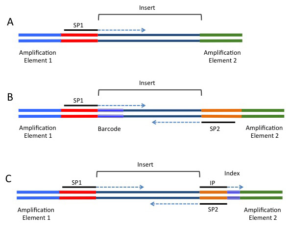
Table 3.1 List of functional elements contained in sequencing adapters.
| Adapter element | Requirement | Location | Function |
| Amplification element | Required | 5′ and 3′ terminus | Clonal amplification of the construct |
| Primary sequencing priming site | Required | Adjacent to the insert | Initiating the primary sequencing reaction |
| Barcode/Index | Optional | 5′-end of the insert/Between the sequencing priming site and its respective amplification element | Provides a unique label to sequences from different samples. Allows pooling of multiple experiments in a single sequencing reaction. |
| Paired-end sequencing priming site | Optional | Adjacent to the insert on the side opposite of the primary sequencing priming site | Sequencing into the insert on the end opposite of the primary read |
| Index sequencing priming site | Optional | Complementary to the 5′-end of the sequencing priming site | Sequencing of the index |
3.5.1 Multiplexing samples with barcodes/indicies
Copy this link to clipboard
Most high-throughput sequencers produce many millions of sequence reads in a single reaction. In some cases the number of reads that can be obtained can exceed the needs of the experiment. Considering time and expense it is often desirable to pool ("multiplex") libraries from multiple experiments into a single sequencing reaction. To identify which experiment a given sequence comes from, each library is prepared using adapters containing different tags (commonly known as an index or barcode). The tags are typically short (5-7 bp) sequences that are read during sequencing. The sequence of the insert and tag can then be associated, allowing one to identify which sample the insert came from.
More on barcodes and indicies
More on barcodes and indicies
Two kinds of sequence tags are commonly used.
Barcodes: The first (typically known as a barcode, or "inline barcode") is located in between the sequence priming site and the insert (see Figure 3.2). Sequence reads obtained using this configuration therefore contain the barcode followed by the insert. User created scripts or various available software packages can be used to sort the sequence reads by their barcode.
With some platforms problems can arise if one uses few or very similar barcodes. Be sure to consult with your sequence provider before attempting to use this multiplexing approach.
Indices: The Illumina sequencing platform also supports a second type of tag (typically known as an index, or "inline index"). The index is located within the 3′-adapter and is read using a separate sequencing reaction that follows the primary sequencing reaction. The Illumina sequencing software (and/or many independent read processing programs) then makes the association between the read and the individual library from which it came.
3.5.2 Paired-end sequencing
Copy this link to clipboard
Most current techniques are only capable of producing accurate sequence reads of 50 - 300 bases which is often less than the length of the insert. In order to increase the sequence coverage of inserts most platforms allow inserts to be sequenced from both ends. This technique (known as paired-end sequencing) can be used to increase the mapping accuracy and provides information that is useful for isoform detection. In order to use paired-end sequencing the adapters must contain a sequencing priming site that is situated on the opposite side of the insert (see Figure 3.2).
This option is supported by most of the current sequencing platforms but be sure to consult with your sequencing provider before designing experiments that utilize paired-end reads.
3.6 Addition of adapters
Copy this link to clipboard
As discussed above, platform specific sequences must be present at the end of the fragments before they can be sequenced (as shown in Figure 3.2). Several strategies have been developed for adding adapter sequences to create the asymmetrical molecule.
More on addition of adapters
More on addition of adapters
3.6.1 Addition of adapters via Y-adapter PCR
Copy this link to clipboard
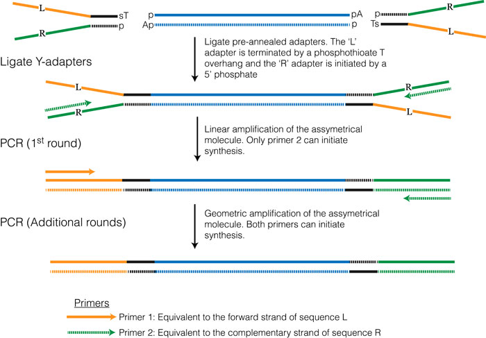
This method is one of the most commonly used and is essentially the same method that was developed for high-throughput sequencing of genomic DNA. Once the RNA is converted to double stranded cDNA the ends are blunted and adenosine overhangs are added. The adapter sequences can be added using a technique commonly referred to as Y-adapter PCR (see Figure 3.3).
Figure 3.3
3.6.2 Addition of adapters via RT/PCR
Copy this link to clipboard
Specific sequences can be added to each end of the insert during the first- and second-strand synthesis steps. In this case the reverse transcriptase primer can contain an overhanging sequence that doesn't anneal to the RNA template but contains at least a portion of the adapter sequences corresponding to those shown on the right in Figure 3.2. In a similar manner the forward PCR primer can contain over-hanging sequences corresponding to those shown on the left in Figure 3.2. Two kits (SMARTer and ScriptSeq) use this approach, and both employ proprietary chemistries and primer sequences.
3.6.3 Addition of adapters via ligation
Copy this link to clipboard
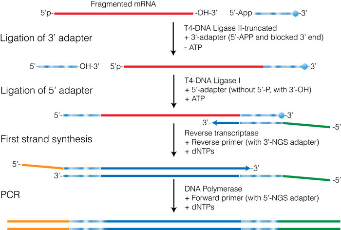
Although the technical details differ, this approach is used in the Illumina TruSeq Small RNA kit, the NEBNext Small RNA prep kit, and in the SOLiD RNA kits from Life Technologies. These kits use ligation procedures that allow two different adapters to be ligated onto each end of the target RNA. These adapters are then used to prime the first- and second-strand synthesis reactions resulting in cDNAs terminated by the appropriate adapter sequences.
Figure 3.4 shows an outline of the procedure used in both the Illumina TruSeq and in the NEBNext small RNA prep kits. The first step involves ligating an oligo to the 3′-OH of the RNA and takes advantage of the enzymatic activity of T4 RNA ligase II-truncated (T4 Rnl2-trunc) which is a modified form of T4 RNA ligase II. This enzyme can specifically ligate an oligo possessing a 5′-pre-adenylation group to RNA with a 3′-OH. Unlike the full-length ligase, T4 Rnl2-trunc is unable to adenylate the 5′-end of the RNA, preventing circularization of the RNA molecule.
The 5′-adapter is then admixed with T4 RNA ligase and ATP, all of which promotes ligation of the 5′-adapter onto the 5′-end of the RNA. One of the biggest challenges with this procedure is the formation of 5′-adapter-3′-adapter products that can form during the second reaction. In the NEBNext Small RNA prep kit this reaction is quenched by the addition of the RT-primer before the second ligation step. The RT-primer is a DNA oligo that contains sequence complementary to the 5′-end of the 3′-adapter oligo. Free 3′-adapters therefore form a double-stranded molecule that is unable to act as a substrate for the ligation reaction.
Figure 3.4
3.7 Preparation of stranded libraries
Copy this link to clipboard
Conventional RNA-seq library protocols involve converting the RNA to double-stranded cDNA followed by the ligation of sequencing adapters. Although Y-adapter PCR results in an asymmetrical molecule, in reality the final libraries contain two populations of molecules with respect to the original RNA template. In one population the strand that is sequenced corresponds to the sense strand while in the other the strand that is sequenced corresponds to the anti-sense strand. Thus the 'strandedness' of the original RNA template is lost.
Why does this matter? Knowledge of which strand a read comes from may not be critical for measuring differential gene expression since most read aligners (see "Aligning RNA-seq reads to a reference") have settings that allow them to evaluate both the initial read and its reverse-complement. However, for genomes in which transcribed regions overlap (not most eukaryotic organisms), knowledge of strandedness may help assign reads to genes adjacent to one another but on opposite strands. In addition, if one is primarily interested in annotation strandedness can be used to discover features such as the existence of overlapping anti-sense transcripts.
More on stranded protocols
More on stranded protocols
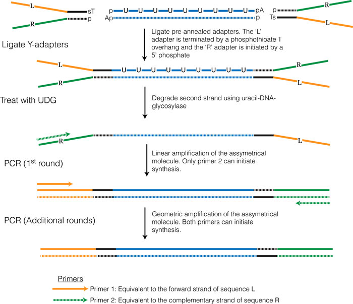
Various 'strand-specific' library preparation protocols have been developed and several of these were reviewed in Levin et.al. 2009. The method that has become the most popular (and performed well according to Levin et.al. 2009) takes advantage of the fact that E. coli DNA polymerase can synthesize DNA using either dUTP or dTTP. In this protocol dUTP is used for synthesis of the second strand, which essentially marks this strand. Y-adapters are then ligated onto both ends in the same manner as in the non-strand-specific protocol. Two approaches have been developed to selectively amplify the non-dUTP strand. One approach (see Figure 3.5 below and outlined in Borodina et al. 2011) involves adding uracil-DNA-glycosylase (UDG) which cleaves the second strand where dUTP has been incorporated, effectively preventing this strand from being amplified during the subsequent PCR amplification. The second approach (which is currently used in the Illumina TruSeq Stranded RNA-seq library preparation kit) involves using a DNA polymerase that is incapable of extending past dUTP bases.
Figure 3.5
3.8 Validation and Quantification
Copy this link to clipboard
To achieve the highest quality of data, it is important to validate the quality and accurately quantify the cDNA libraries before sequencing. As discussed in the RNA preparation section, each of the commonly used methods has certain drawbacks. Absorbance-based methods can lead to erroneous measurements due to residual primers and dNTPs and may not be sensitive enough to accurately measure the library concentrations if the library yield is low. Fluorescence-based techniques generally are more sensitive to RNA concentration but less sensitive to contaminants. If multiplexing multiple libraries in a single sequencing reaction, make sure to adjust the relative contributions from each library to suit your experimental design needs. Other robust options for quantification include quantitative PCR (qPCR) and estimation of fragment concentration using electrophoretic instruments like the ABI Bioanalyzer.
Assessing the fragment size distribution of final RNA-seq libraries is also important. The sizes of the molecules should fall into the expected size range (depending on protocol), and the libraries should be free of ligation/PCR artifacts (usually small relative to the desired molecules). Fragment sizes can be evaluated via electrophoresis, preferably using a sensitive instrument such as an ABI Bioanalyzer.
4. Sequencing
Copy this link to clipboard
-
Design ExperimentSet up the experiment to address your questions.
-
RNA PreparationIsolate and purify input RNA.
-
Prepare LibrariesConvert the RNA to cDNA; add sequencing adapters.
-
SequenceSequence cDNAs using a sequencing platform.
-
AnalysisAnalyze the resulting short-read sequences.
4.1 Overview
Copy this link to clipboard
Sequencing technologies are rapidly expanding and new sequencing chemistries are being developed at a rapid pace. A number of sequencing platforms are widely available, including Illumina, Ion Torrent, and PacBio. The first nanopore sequencing devices are now being marketed by Oxford Nanopore while several legacy technologies can still be found, including Life’s 454 and SOLiD. Each is based upon different proprietary chemistries and technologies and each has unique strengths and weaknesses. A good overview of several platforms is provided by Metzker (2009).
4.2 Choosing a sequencing platform
Copy this link to clipboard
One of the first steps that must be done when designing an RNA-seq experiment is choosing a sequencing platform. It is critical to understand that short-read sequencing requires the addition of specific adapter sequences to the ends of the cDNA molecules of interest. (This is covered in more detail under "Library Preparation"). Since each platform uses unique proprietary adapters the correct adapters must be added to match the sequencing platform.
Although many sequencing platforms exist some are better suited for RNA-seq than others. The current leading platform for RNA-seq is Illumina. This platform enables deep sequencing which is generally important for RNA-seq, and provides long enough, low-error reads that are suitable for mapping to reference genomes and transcriptome assembly. For detailed comparisons of the available platforms see Liu et al. (2012) and Glenn (2011). A useful online comparison can be found at bluseq. The PacBio platform is also beginning to be used for transcriptome assembly, although its use is still in the early stages. Each read from a PacBio is often long enough to recapitulate a full length cDNA transcript.
4.3 Sample preparation and submission
Copy this link to clipboard
Before initiating an RNA-seq experiment users should first consult with the sequencing facility they intend to use to make sure they understand the sample preparation and submission requirements. Some general issues that need to be considered are:
- That the samples are clean and free of major contaminants.
- The primary DNA molecules contain inserts of the correct size.
- The primary DNA molecules have adapters on each end.
- The sample concentration is appropriate.
- The samples are suspended in appropriate buffers.
Furthermore, the facility needs to know:
- The sequence of the sequence-priming site.
- The length of the read you desire.
- Whether you want single-end or paired-end reads.
- Whether there is a barcode or index sequence.
- If using Illumina sequencing the facility also needs to be notified if the inserts contain a region of low sequence complexity immediately after the sequence-priming site (i.e. a barcode).
5. Analysis
Copy this link to clipboard
-
Design ExperimentSet up the experiment to address your questions.
-
RNA PreparationIsolate and purify input RNA.
-
Prepare LibrariesConvert the RNA to cDNA; add sequencing adapters.
-
SequenceSequence cDNAs using a sequencing platform.
-
AnalysisAnalyze the resulting short-read sequences.
5.1 Overview
Copy this link to clipboard
The analysis and interpretation of genomic data generated by sequencing are arguably among the most complex problems modern scientists face. A staggering degree of effort by biologists, computer scientists, mathematicians, and statisticians is currently leveled at curating, manipulating, and interpreting this information. RNA-seq is subject to many of the same issues other sequencing applications face, in addition to some nuances. Please keep in mind that the nature of questions people may address using RNA-seq data is effectively limitless, so there are even more facets to the analysis of transcriptomes than there are to generating the data itself. As a disclaimer, we emphasize that it is virtually impossible to stay abreast of all developments in approaches to analyzing RNA-seq data. Our objective rather is to provide in the following outline a rough guide to commonly encountered steps and questions one faces on the path from raw RNA-seq data to biological conclusion.
To generalize, however, embarking on an RNA-seq study usually requires initial filtering of sequencing reads, assembling those reads into transcripts or aligning them to reference sequences, annotating the putative transcripts, quantifying the number of reads per transcript, and statistical comparison of transcript abundance across samples or treatments.
Stereotypical RNA-seq Analysis Pipeline
- Demultiplex, filter, and trim sequencing reads.
- Normalize sequencing reads (if performing de novo assembly)
- de novo assembly of transcripts (if a reference genome is not available)
- Map (align) sequencing reads to reference genome or transcriptome
- Annotate transcripts assembled or to which reads have been mapped
- Count mapped reads to estimate transcript abundance
- Perform statistical analysis to identify differential expression (or differential splicing) among samples or treatments
- Perform multivariate statistical analysis/visualization to assess transcriptome-wide differences among samples
5.2 Initial processing of sequencing reads
Copy this link to clipboard
Before either de novo assembly or alignment of RNA-seq reads to a reference, they must be processed for a number of reasons described in this section.
Outline:
- Demultiplex by index or barcode
- Remove adapter sequences
- Trim reads by quality
- Discard reads by quality/ambiguity
- Filter reads by k-mer coverage
- Normalize k-mer coverage
Please see Table 5.1 for examples of programs developed to address these steps.
5.2.1 Demultiplexing by index
Copy this link to clipboard
Many researchers multiplex molecular sequencing libraries derived from several samples into a single pool of molecules read by the sequencer. Multiplexing is a common strategy due to the sheer amount of data a sequencer is able to generate. A single flow cell lane from an Illumina HiSeq 2000 instrument, for example, routinely yields 150 million sequences. Most RNA-seq libraries do not require that level of coverage, so it makes sense to combine samples to save costs. Multiplexing of samples is made possible by incorporation of a short (usually at least 6 nt) index or "barcode"; into each DNA fragment during the adapter ligation or PCR amplification steps of library preparation. After sequencing, each read may be traced back to its original sample using the index sequence and binned accordingly. Depending on the library preparation method and sequencing technology, the sequencing instrument software may or may not perform the partitioning. For example, Illumina TruSeq technology incorporates an index that is sequenced as a separate read for each flow cell cluster, which may be used by the sequencing software to demultiplex reads before delivery to the end user. If you submit an index multiplexed library to your Illumina sequencing facility, let them know about it and provide them with a list of the index sequences in each pool. In other cases, inline barcodes incorporated as part of the sequencing adaptor(s) are part of the sequencing read itself, and these data are demultiplexed (and the barcodes are trimmed off the reads) by the user after sequencing. Important considerations to make when using inline barcodes include using barcodes that are far enough apart in sequence space to be reliably distinguished from one another in the face of sequencing errors and, in the case of Illumina sequencing, using barcodes that are variable across samples at the first few bases to ensure adequate cluster discrimination. Many programs have been written to demultiplex barcoded library pools, some of which are presented in Table 5.1.
5.2.2 Removing adapters
Copy this link to clipboard
If cDNA insert sizes are sufficiently small and sequencing read lengths sufficiently long, it is possible to generate sequencing reads that contain a portion of adapter sequence at the 3′-end. Therefore, depending on the library preparation method and range of cDNA insert sizes, it may be prudent to trim these artifacts away. Removing these artifacts should improve assembly and/or mapping of sequencing reads. Again, several pieces of software have been developed independently to address this issue, and a subset is referenced in Table 5.1.
5.2.3 Filtering/Trimming reads by quality
Copy this link to clipboard
Many end users also elect to discard reads suspected to contain sequencing errors. Reads likely to contain multiple sequencing errors provide less biological information and are expected to hinder assembly and alignment. Some analyses are more tolerant of error than others. For example, de novo assembly requires much cleaner reads than alignment to a reference genome. A common filtering step along these lines is to discard or trim reads containing low quality bases. Reads generated on the Illumina platform are known to have a higher error rate as you move towards the 3′-end of the read, so if a drop in quality is detected within the read, it is normal to trim the rest of the read off. Absolute minimum, average, and sliding-window-average quality scores are commonly used as criteria for discarding and/or trimming reads.
Just how output from the sequencer is translated to base call quality (i.e. the probability of a correct call), depends on the sequencing platform and the version of base-calling software. The sequencing reads, along with the corresponding base call qualities are delivered to the user typically as a FASTQ file (which has the extension ".fastq" or ".fq"). These FASTQ files contain a four-line record for each read, including its nucleotide sequence, a "+" sign separator (optionally with the read identifier repeated), and a corresponding ASCII string of quality characters. Each ASCII character corresponds to an integer i ranging from -5 to 41 (depending on the version of Illumina software used for base-calling), and may be translated to p, the probability that a given base is incorrectly called, using either the "Phred" scale where i = -10*log10(p), or a modified scale where i = -10*log10[p/(1-p)], again, depending on the version of base-calling software used by the sequencer (Cock et al. 2010). For a more detailed description, please see the fastq format Wikipedia page: http://en.wikipedia.org/wiki/FASTQ_format.
Legacy sequencing platforms, such as Life Technologies' SOLiD or Roche's 454, among others, generate a variety of file formats. There are a number of tools available to convert these files to FASTQ format which is the standard used by most bioinformatic tools.
5.2.4 Filtering/Normalizing Reads by k-mer Coverage
Copy this link to clipboard
If assembling tens of millions of RNA-seq reads de novo into a reference assembly is a necessary step in your analysis pipeline, we recommend the use of k-mer distribution statistics to normalize and potentially screen your data first. K-mers are length k substrings of the DNA sequences in a dataset and are a computationally tractable way of representing the information contained in that dataset. K-mer dictionaries can be built from a set of reads and ultimately used to address issues such as redundancy, sequence variants, and errors among reads. Manipulation of short-read sequencing data according to k-mer coverage is a valuable idea (Brown et al. 2012), and there are several useful tools for implementing it. K-mer-based management of short-read data becomes necessary primarily because graph-based de novo assembly approaches (see assembly section) perform poorly in the face of sequence variation within (and uneven coverage among) the discrete units of assembly, which in the case of RNA-seq data are transcripts.
As it turns out, sequencing errors (and real variants owing to polymorphism and mutation) can throw off graph-based assembly algorithms. In light of this concern, it may be a good idea to eliminate reads with grossly non-uniform k-mer coverage. For example, a read containing a sequencing error may escape quality score-based filtering steps. Because sequencing errors are relatively rare we expect the erroneous base in this read to manifest itself as a "dip" in the dataset-wide abundance of k-mers along the read, specific to the location of the k-mers containing the error. By detecting such islands of rare k-mers in reads, the reads can be flagged for removal from the dataset to improve de novo assembly. The flexible kmer_filter module of the Stacks pipeline (Catchen et al. 2011) can implement this type of specialized filtering, in addition to global filtering by rare, abundant, or both k-mer types.
Uneven coverage among transcripts may be remedied by discarding reads until k-mer frequencies are brought down to a specified threshold, one that is approximately minimal for de novo assemblers to work optimally. This process is known as "digital normalization", and in general researchers have found that normalizing to an average k-mer coverage of 20-30X often works well for de novo assembly (Brown et al. 2012). As always, we recommend exploring parameter space with each new data set. Perhaps surprisingly but often, one will be able to reduce his or her sequencing reads to 10% of the original quantity and obtain a transcriptome assembly much faster than (and superior to) an assembly based on the full data set. The k-mer tool package khmer from Titus Brown's lab enables normalization to a specified median k-mer coverage, among other handy, k-mer-based manipulations of short-read sequencing data.
Table 5.1 Read Processing Software
| Software | De-mulitplexing | Adaptor Trimming | Quality Filtering/ Trimming | K-mer Filtering | K-mer Normalization |
| FASTX-Toolkit | |||||
| Goby | |||||
| khmer | |||||
| NGS_backbone | |||||
| Stacks | |||||
| trimmomatic | |||||
| biopieces |
5.3 De novo Transcriptome Assembly
Copy this link to clipboard
If you can't align RNA-seq data to a well-assembled reference genome from a relatively recently diverged organism, building a reference transcriptome out of RNA-seq reads is an alternative strategy. The primary goal in assembling a transcriptome de novo is to reconstruct a set of contiguous sequences (contigs) presumed to reflect accurately a large portion of the RNAs actually transcribed in the cells of your organism. This turns out to be no trivial task, because a limited amount of information about the original gene transcripts is retained in the short reads produced by a sequencer. The assembly process must place reads from the same transcript together in the face of variants introduced by polymorphism and sequencing errors, and the process must assemble reads from different but often similar, paralogous transcripts as separate contigs. Furthermore, repetitive regions that exist within genomes make assembly especially difficult, although this is probably less of a problem for transcriptome assembly than genome assembly.
The building of reference transcritpomes is a powerful way to discover and annotate transcribed regions of a genome. It is also possible, and a common desire, to align RNA-seq reads to an assembled transcriptome for quantification and comparison of transcript abundance among samples. If the latter is your objective, keep in mind that the reference transcriptome you assemble should be representative of transcripts whose expression levels you are interested in interrogating. For example, you wouldn't want to assemble a reference transcriptome using RNA-seq data derived from the gut of your organism, and then try to compare transcript abundance between ovary and testis samples by mapping reads derived from those tissues. Also keep in mind that the transcriptome of many tissues is extremely heterogeneous with respect to the abundance of individual transcripts. Due to this non-uniform distribution we often end up with copious amounts of data for a relatively small subset of genes, and sparse data for many genes expressed at low levels. One solution to this is to prepare a library using RNAs derived from multiple tissues or developmental stages, and then normalize the cDNA using DSN (see target enrichment) before sequencing.
Other important considerations to make when generating data for a reference transcriptome assembly are sequencing platform and read length. While there is arguably no single best type of data for a de novo transcriptome assembly, most have found that a combination of longer reads and high sequencing depth yields the best results. For example, generating 100 million or more, longer (e.g. 100 nt) Illumina paired-end reads will strike this balance. Alternatively, a mixture of shorter, high-throughput SOLiD and longer, lower-throughput 454 reads may converge on the same optimum. Read length and coverage do matter when it comes time to assemble the transcriptome, however, as different de novo assemblers employ different approaches that depend heavily on these parameters. A newer method involves using the PacBio platform to generate long sequencing reads (typicaly 1-10kb in length). The PacBio sequencer is generally able to generate a full, novel transcript with each read produced on the platform.
Here we do not attempt to present a detailed, comprehensive review of how de novo assembly works, nor do we dissect the nuances of different assembly approaches. Other published reviews have tackled these topics. Solutions to sequence assembly arose from the field of mathematics known as graph theory. For general reviews of how genomic sequencing data is assembled using graphs, see (Miller 2010; Compeau 2011; Li 2011). For a specific review of transcriptome assembly, see (Martin and Wang 2011), and for comparisons of how choice of assembly software and sequencing depth affect de novo transcriptome assemblies, see (Brautigam 2011; Francis 2013). Below we summarize at a superficial level the general approaches currently used for de novo transcriptome assembly, along with examples of commonly used software. These approaches were designed with genome assembly in mind but have been adapted for transcriptome assembly as necessary. Finally, we provide a basic comparison of actual de novo transcriptome assemblies for a non-model teleost (pipefish), specifically addressing assembler differences as a function of contig length.
5.3.1 de Bruijn Graph-Based Assembly
Copy this link to clipboard
This type of solution to assembly has been around since the era of Sanger data (Pevzner, Tang, Waterman 2001), but has since been adapted to accommodate the millions of short sequencing reads encountered during today's assembly projects. Instead of laboriously aligning all pairs of reads in a data set to layout the overlap structure, de Bruijn graph approaches first break each read into its constituent substrings of length k (k-mers). There are fewer total unique k-mers in a large set of short reads than there are unique reads, so building graphs based on k-mer, as opposed to read overlaps, simplifies things computationally. Also, de Bruijn graph assemblers generally try to find a different type of path through graphs (a Eulerian path) based on k-mer overlap than the path typically solved for reads during OLC assembly. In general, a de Bruijn approach constructs a graph in which k-mer overlaps form the nodes, edges connecting overlaps represent the k-mers themselves, and the path through the graph must visit each edge once (Compeau, Pevzner, Tesler 2011). For details regarding the specific algorithms used to implement de Bruijn graph approaches to assembly, consult the primary publication(s) associated with each piece of software. Below we list and briefly describe five commonly used de novo transcriptome assemblers based on de Bruijn graphs. For higher coverage RNA-seq data (e.g. Illumina and SOLiD), de Bruijn assemblers are necessary, but they may be used successfully for lower coverage RNA-seq data as well.
5.3.1.1 Commonly used graph-based assembly software
Copy this link to clipboard
Velvet/Oases: Velvet (Zerbino, Birney 2008) is a sophisticated set of algorithms that constructs de Bruijn graphs, simplifies the graphs, and corrects the graphs for errors and repeats (especially well if paired-end reads are used). The user can specifiy minimum contig coverage and the k-mer length.
Oases (Schulz et al. 2012) post-processes Velvet assemblies (minus the repeat correction) with different k-mer sizes. Different k-mer sizes are used to ensure that more space of the k-mer size / coverage relationship is explored, given that transcriptomes are inherently non-uniformly covered. Sets of contigs in the final assembly often represent different isoforms of the same locus. A merged assembly from all k-mer lengths may be produced as the final result to reflect a consensus across multiple assemblies. Velvet and Oasis are available at: www.ebi.ac.uk/~zerbino/velvet/ and www.ebi.ac.uk/~zerbino/oases/.
Trans-ABySS: Much like the Velvet/Oases model, Trans-ABySS (Robertson et al. 2010) takes multiple ABySS assemblies (Simpson et al. 2009) produced from a range of k-mer sizes to optimize transcriptome assemblies in the face of varying coverage across transcripts. ABySS and Trans-ABySS were designed to run in a highly parallelized fashion to accommodate especially large data sets. Trans-ABySS is available at: www.bcgsc.ca/platform/bioinfo/software/trans-abyss.
Trinity: Trinity (Grabherr et al. 2011) produces a transcriptome assembly through three steps, which correspond to discrete modules named "Inchworm", "Chrysalis", and "Butterfly", Inchworm builds initial contigs by finding paths through k-mer graphs, each contig assembly seeded by k-mers in order of k-mer abundance. Chrysalis groups these contigs together given sufficient k-mer overlap and builds de Bruijn graphs for these groups, in which the overlaps are nodes and the k-mers connecting edges. Butterfly simplifies the graphs when possible, then reconciles the graphs with original reads (or read pairs) to output individual contigs representative of unique splice variants and paralogous transcripts. It is available at: trinityrnaseq.sourceforge.net.
Currently, the most commonly used assemblers are Velvet/Oases and Trinity.
5.3.2 Overlap-layout-consensus assembly
Copy this link to clipboard
This approach to de novo assembly was originally used to assemble Sanger-generated sequences into contigs for both genome and EST (expressed sequence tag) reconstructions.
More on OLC assembly
More on OLC assembly
Overlap-layout-consensus (OLC) assembly first obtains explicit overlap information for all reads by pairwise alignment (aided heuristically by initial grouping of reads according to k-mer content). Second, a graph is constructed, in which individual reads are represented by "nodes", which are connected by "edges" that represent the overlaps. A "Hamiltonian" path (Compeau 2011) through the graph, in which each node is visited only once, is traversed, and the non-overlapping bases between two consecutive nodes for every step in the path are concatenated to form the assembled contig. For data sets that consist of hundreds of millions reads, the iterative pairwise-alignment step in this approach is not computationally feasible. Furthermore, finding the path through this particular type of graph is exceedingly difficult when the graph is very large (very large graphs can result from high-coverage data owing to more reads and more sequencing errors). Consequently, OLC assembly is best suited to lower coverage, longer read data such as Sanger, 454, or PacBio.
5.3.2.1 Commonly used OLC assembly software
Copy this link to clipboard
CAP3: CAP3 (Huang and Madan 1999) was developed primarily to assemble genomes but has been used for EST assembly as well. It has quality-based read-end trimming capabilities and makes use of base quality scores during all alignment steps during assembly. It is available at: http://seq.cs.iastate.edu/
MIRA 3: The MIRA assembly model (Chevreux 2004) has undergone several major changes over the years. The current version is suitable for genome or transcriptome assemblies, handles single or paired-end Sanger, 454, Illumina and hybrid data sets, and makes use of base quality scores. It is available at: http://sourceforge.net/apps/mediawiki/mira-assembler/index.php?title=Main_Page
Roche GS De Novo Assember ("Newbler"): This suite of software, which contains an assembly tool specifically for transcriptome assembly, is available through Roche (http://454.com/products/analysis-software/index.asp). The algorithms are tailored to 454 data, and are reported to handle elevated homopolymer sequencing error rates especially well. For transcriptome assemblies, this software attempts to assemble differentially spliced transcripts (different sets/orders of exons) as separate contigs, grouped as "isotigs".
5.4 Aligning RNA-seq reads to a reference
Copy this link to clipboard
Short reads generated by RNA-seq experiments must ultimately be aligned, or "mapped" to a reference genome or transcriptome assembly. Read alignment to a reference provides biological information in two basic ways. First, it generates a dictionary of the genomic features represented in each RNA-seq sample. That is, aligned reads become annotated, and the highly fragmented data is thus connected to the gene families, individual transcripts, small RNAs, or individual exons encompassed by the original tissue sample. Second, the number of reads aligned to each feature approximates abundances of those features in the original sample. Such measures of digital gene expression are then subject to comparison among samples or treatments in a statistical framework.
Please be aware that if you used digital normalization of RNA-seq reads in preparation for de novo assembly, but now want to quantify transcript abundance, you need to align the original cleaned reads (not the normalized ones) to the transcriptome.
The general objective when mapping or aligning a collection of sequencing reads to a reference is to discover the true location (origin) of each read with respect to that reference. Obviously features of the reference such as repetitive regions, assembly errors, and missing information will render this objective impossible for a subset of the reads. Likewise, sequencing errors, polymorphisms, and limited complexity within the short reads will make them harder to align. In light of these factors, aligners must be flexible when applying mapping criteria. That is, they must allow for approximate matches. Otherwise, a large proportion of sequencing reads will not be assigned to a particular feature in the reference. Just how "approximate" the matches are depend on the features of the aligner, usually manifested as user-specified parameters such as the proportion of bases in each read required to match the reference identically, and penalties incurred by insertions, deletions, and gap sizes. There is no easy answer to which aligner one should choose or which alignment parameter values one should select for a particular aligner. Like many other steps in RNA-seq analysis, there really is no substitute for a little exploration of parameter space. Obviously alignment parameter settings that are extremely stringent will result in a small subset of your reads being mapped. Very liberal settings, on the other hand, will result in lost specificity, and many reads will map to multiple features of the reference. It therefore takes a little bit of experimentation to get the optimal balance of sensitivity and specificity for a given data set.
There is no short supply of short read aligners. In fact, dozens have been developed within the last several years, and some (but not all) were designed with specific utilities in mind. Several effective and popular aligners include Bowtie2, BWA-mem, and GSnap. Fonseca et al. 2012 maintain an updated, near-comprehensive database of aligners here. In the following section we outline several broad categories into which short read aligners fall, specifically with respect to RNA-seq. Keep in mind that using alignment software generally requires two basic steps. First, the reference genome or transcriptome (generally in ".fasta" format) is converted to an indexed "reference" by the software in order to allow fast read mapping, which is the second step. Both building the reference and aligning sequencing reads are usually quite straightforward given specific instructions in software manuals/websites. Depending on the speed of the aligner (some are much slower than others) and the number of reads you have to align, consider breaking up reads into multiple files and running alignments in parallel, across multiple nodes on a computer cluster, for example.
5.4.1 Aligning to a reference genome
Copy this link to clipboard
If you are mapping your reads to a reference genome, you need an alignment tool that can allow for a read to be "split" between distant regions of the reference in the event that the read spans two exons. Since the sequencing library was constructed from transcribed RNA, intronic sequence was not present, and the sequenced molecule natively spanned exon boundaries. When aligning back to a reference genome we have to account for reads that may be split by potentially thousands of bases of intronic sequence. Some spliced aligners split reads across exons from no additional information (de novo spliced alignment), while others need intron/exon boundary annotations from the reference genome. Typically the intron/exon annotations are available in a GFF3 file or a GTF file. These files are usually available for download at the same location that you obtained your reference genome. Including intron/exon annotations with your RNA-seq alignment will significantly improve the quality of the alignments. Of course, if you are annotating a new genome assembly using your RNA-seq reads, you will need to use an aligner that can do de novo splicing -- and most aligners can operate with or without annotation.
5.4.2 Aligning to a transcriptome
Copy this link to clipboard
If you are mapping reads to a transcriptome intron/exon boundaries are irrelevant. However you may still need to worry about gapped alignments depending on the type of transcriptome you assembled. There are two basic strategies to transcriptome assembly: 1) assemble a single, longest gene model for each set of splice variants, and 2) try to reconstruct each variant separately. In the former case, you will still need to map reads from splice variants that span exon boundaries in your single gene model. In the later case, all of your reads should be contiguous so you don't need to worry about gaps. However, it is much more difficult to assemble all variants accurately, so many researchers prefer to assemble a single, longest gene model.
5.4.3 microRNA aligners
Copy this link to clipboard
Some aligners are designed to map especially short sequences, such as those obtained from mircoRNA-seq studies. These aligners include parameter value ranges necessary for the optimal alignment of reads that are only 16-30 nt. If you're working with microRNA reads, consider using one of the following:
- MicroRazerS (www.seqan.de/projects/microrazers/)
- mrFAST (mrfast.sourceforge.net/)
- mrsFAST (mrsfast.sourceforge.net/Home)
- PatMaN (bioinf.eva.mpg.de/patman/)
5.4.4 Output files from short read aligners
Copy this link to clipboard
The results of short read alignments are very commonly summarized and output in the form of SAM files, or BAM files (the compressed, binary equivalent of SAM). These files should contain all of the information you need for downstream analyses such as annotation, transcript abundance comparisons, and polymorphism detection. For a description of the SAM format see samtools.sourceforge.net/SAM1.pdf. The software suite SAMtools (Li et al. 2009) provides a convenient platform for the manipulation of SAM and BAM files. In a SAM file, each alignment (each match according to the constraints imposed by the aligner), is represented on a single line. Information fields associated with each alignment exist as columns in the file and include the read name, the feature of the reference to which the read aligned, the position of the alignment, and a numerical quality score of the alignment, etc.
A common and logical method to estimate transcript abundance across a reference transcriptome using RNA-seq data is to count the number of reads that map uniquely to each transcript. Reads that map to multiple contigs or transcripts may provide ambiguous information and therefore introduce more noise than is desirable in some contexts. If, on the other hand, alternative splice variants are separate features in the reference, one would expect multiply mapped reads and may want to count them, but in an unbiased manner. In any case, it is straightforward to count the number of reads aligned to each reference feature from a SAM file, write a tabular file containing this information, and use this file for differential gene expression analysis (see the section Differential gene/isoform expression). The package Picard (available at picard.sourceforge.net/) is a useful companion to SAMtools, and will enable additional manipulations of BAM files (e.g. the acquisition of only uniquely mapped reads).
5.5 Annotation of transcripts
Copy this link to clipboard
Most people are interested in the identities of the transcripts they assemble or identify as differentially expressed or alternatively spliced. Annotations connect novel RNA-seq data with biological information about the same (or homolgous) transcripts derived from other studies. For example, it is important to identify gene families or known pathways that respond transcriptionally to specific experimental treatments. Also, RNA-seq data derived from eukaryotic organisms may contain reads from other species (parasites, for example), and one would want to know about this.
In the event that a reference genome is available, annotation is relatively straightforward. Genomic coordinates from the reference genome are normally associated with various forms of annotation information through databases such as genome browsers. Given mapping coordinates from an alignment, for example, it is possible to extract the corresponding information from such databases.
A transcriptome assembled de novo, on the other hand, is often annotated from scratch. The most common way to annotate transcripts in this situation is to use the NCBI-supported BLAST (Basic Local Alignment Search Tool) (Altschul et al. 1990), the recent, widely used suite of tools being "BLAST+" (Camacho et al. 2009). A description of the BLAST+ command line applications can be found at www.ncbi.nlm.nih.gov/books/NBK1763/. In essence, the BLAST model allows the user to "match" query sequences to one or more databases of curated, annotated sequences, using an efficient local sequence alignment approach. In some situations it may be adequate to blast contigs against a database of known or predicted transcripts from the reference genome of a closely-related organism. In other situations it may be desirable to blast contigs against all nucleotide sequences in an inclusive database, such as the NCBI nucleotide database ("nt"), which itself is composed of entries from smaller databases. If the annotation emphasis is on protein-coding transcripts, BLASTx, which translates each query sequence (in all six reading frames) to amino acid sequences and uses these to query a protein database, is an appropriate tool. All NCBI databases are available at ftp.ncbi.nlm.nih.gov/blast/db/.
Once an automated BLAST search has been performed for a collection of sequences (contigs from a reference transcriptome, for example), one of several specifiable output formats may be parsed to extract information about the number of "hits", the probability that the alignment of a query to each hit occurred by chance (the "e-value"), the descriptions and accession numbers for each hit, and representations of the sequence alignments themselves. This information may then be used in a variety of ways, including basic annotation, evaluation of redundancy in the assembly, or functional enrichment analyses.
One generally useful way to compare groups of transcripts or contigs that are differentially expressed or otherwise is through Gene Ontology (GO) term analysis (www.geneontology.org/GO.doc.shtml). Entries in sequence databases such as those from NCBI are associated with a number of biologically relevant terms. The terms belong to one of three basic "ontologies:" cellular component, biological process, and molecular function. These terms are either associated with the database sequences directly via molecular genetic experimental evidence, or indirectly via homology with other sequence entries in the database. It is possible to take the database entry identifiers for a set of blast hits, extract GO term information, and quantify/compare GO term frequencies among different groups of original sequences. Several software platforms accomplish this type of workflow, including:
- Blast2GO (Conesa et al. 2005), available at: blast2go.de/b2ghome
- DAVID (Huang da, Sherman, Lempicki 2009), available at: david.abcc.ncifcrf.gov/
- ermineJ (Gillis, Mistry, Pavlidis 2010), available at: www.chibi.ubc.ca/ermineJ/
5.6 Differential gene/isoform expression
Copy this link to clipboard
The ultimate objective of many RNA-seq studies is to identify features of the transcriptome that are differentially expressed between or among groups of individuals or tissues that are different with respect to some condition. It is important to keep in mind the nature of those "features" to which reads were mapped for counting. If, for example, reads are mapped to a set of references that include different splice variants of the same gene, those splice variants will each be analyzed separately unless treated as a unit. The nature of the features encompassed by read count data depends on what the mapping reference is (e.g. a genome or transcriptome assembly), and what type of aligner was used. Some pieces of analysis software are designed to handle isoform differences (Leng et al. 2013; Trapnell et al. 2013), and others analyze generic features of the transcriptome, so please consider this when selecting both read alignment and differential expression software.
A basic example of differential expression analysis would be the comparison of liver transcriptomes between a group of mice treated with a pharmacological compound and an untreated "control" group. For more details about experimental design in RNA-seq studies, please see the section on Experimental Design. In the past, microarrays were the most commonly used tool for transcriptome-wide interrogation of differential expression. In many contexts microarrays are still the most appropriate choice today, but RNA-seq is a generally more flexible approach. For example, as we have discussed, no previous genomic sequence information from a given organism is necessary for an RNA-seq study, whereas an existing library of expressed sequence tags is required for the construction of expression arrays. Like signals from RNAs hybridized to microarray probes, RNA-sequencing read counts correspond well with actual transcript levels in a sample (Mortazavi et al. 2008). In terms of differential expression analysis, RNA-seq data (counts of mapped reads) are fundamentally different from microarray data (computed scores of image intensity). Unnormalized RNA-seq data, therefore, must be modeled statistically using discrete distributions. In some differential expression analysis methods, however, RNA-seq data are first normalized to account for a number of library- and/or gene-specific biases (explained below), treated as a continuous variable of transcript abundance, and therefore modeled using continuous distributions for statistical inference.
The goal of this section is to provide a brief introduction to the general statistical approaches used to test hypotheses of differential expression, touch on normalization of RNA-seq data and how the statistical approaches implement normalization in a general sense, and provide an annotated list of currently available software for differential gene expression analysis. In lieu of repeating what other authors have accomplished, we refer our audience to several excellent reviews, which go into greater detail regarding the statistical models and test drive many analysis programs with real and simulated data (Bullard et al. 2010; Kvam, Liu, Si 2012; Soneson, Delorenzi 2013).
5.6.1 Normalization of read counts
Copy this link to clipboard
Several factors preclude raw read counts across different libraries (and across genes within the same library) from being compared directly. The most obvious of these affecting cross-library comparisons is sequencing coverage. Two samples sequenced at 10 and 20 million reads but otherwise identical, for example, will be expected to demonstrate 2-fold differences in gene expression on average, even though there are no actual transcriptional differences. Normalizing read counts by coverage is done in a variety of ways, and in many cases differential expression software will implement a method without input from the user. One strategy, for instance, is to divide each gene's read count for a given library by the total number of mapped reads in that library (Oshlack, Robinson, Young 2010). If a handful of differentially expressed genes are extremely abundant, however, this procedure can result in erroneously calling many lowly expressed genes differentially expressed (Bullard et al. 2010). Other approaches normalize by total read counts only from genes expected to be evenly and/or moderately expressed (Robinson, Oshlack 2010). Perhaps the most popular (and robust) class of normalization procedures uses library read count quantiles (e.g. median, 75th percentile, etc.) or related values as scaling factors, as is the case in DESeq (Anders, Huber 2010).
If comparison of expression values among different transcripts is of interest, other normalization factors must be considered. Gene length, for example, influences read counts because more reads per single transcript will be observed for longer genes. The normalization procedure known as "RPKM" (reads per kilobase per one million mapped reads) applies a gene length and library size adjustment (Mortazavi et al. 2008). Although not formally treated in any differential expression software of which we are aware, base content has also been identified as an important among-gene normalization consideration (Oshlack, Robinson, Young 2010). For a detailed, more comprehensive guide to normalization strategies for RNA-seq data, see Dillies et al. 2012 and Bullard et al. 2010.
5.6.2 Differential Expression Analysis: discrete distribution models
Copy this link to clipboard
To estimate transcript abundance of a given target in a given sample, a parameter of interest is the probability that a randomly drawn read (from millions in the library) maps uniquely to that target. If thousands of reads in the library map to the particular target, this probability will be higher than if only a few map, but in general these probabilities will be very low owing to the huge size of the library and the complexity of the transcriptome. These sampling properties are characterized by the Poisson probability distribution, which in principle should enable us to draw inferences about, say, whether the probability that a randomly drawn read from a library of type A maps to transcript X is higher than the probability that a randomly drawn read from library type B maps to transcript X (i.e. differential expression of transcript X between groups A and B).
One issue with RNA-seq data, however, is that the variance of this probability among different individuals of a group is substantially higher than the mean, with respect to many genes (Anders, Huber 2010). A Poisson distribution assumes an equal mean and variance, and is therefore not a good fit. This issue, known as "overdispersion," has inspired statistical software authors to adopt other models, particularly the negative binomial (NB) distribution, which is characterized by an additional dispersion parameter. Several popular differential expression packages, such as edgeR (Robinson, McCarthy, Smyth 2010) and DESeq (Anders, Huber 2010) are based on the NB distribution, but they differ extensively in how the dispersion parameter is estimated, how normalization is performed, or how the hypothesis test is carried out. For a nice tutorial on how DESeq works in these respects, and its actual usage, see: cgrlucb.wikispaces.com/Spring+2012+DESeq+Tutorial.
5.6.3 Differential Expression Analysis: Continuous distribution models
Copy this link to clipboard
Rather than modeling expression estimates as counts, some statistical approaches treat normalized or transformed count values as continuously distributed variables. If these are distributed approximately normally or log-normally, then those distributions may in principle be used for differential expression inferences. Some authors, for example, have compared normalized count data between two groups via t-test (Busby et al. 2013). Because microarray data is continuously distributed, some have used software originally written for array data (Smyth 2004) to analyze normalized RNA-seq data (Soneson, Delorenzi 2013). One upshot of this approach is the ability to use a general linear model framework for more complex experimental designs. For data sets with larger sample sizes (e.g. 5-10), Soneson et al. 2013 found this method to perform especially well.
5.6.4 Differential Expression Analysis: Nonparametric models
Copy this link to clipboard
Nonparametric statistical approaches are especially useful when real data don't conform to specific distributional assumptions. One such approach for RNA-seq data is to calculate a rank-based test statistic (e.g. Mann-Whitney) for differential gene expression between groups. The R software package SAMseq (Li, Tibshirani 2011) adopts this strategy, and uses resampling to get around the issue of unequal library sizes. Nonparametric tests for a variety of experimental design configurations have been derived, so implementing them in differential expression software like SAMseq is convenient. These approaches have proven to be as effective and robust as their parametric counterparts, especially with moderate to high sample sizes (Soneson, Delorenzi 2013).
5.6.5 Choice of analysis software
Copy this link to clipboard
Clearly there are many options when it comes to differential gene expression analysis. Although some packages are more sensitive to some parameters (such as sample size and overdispersion), comparative methods reviews have not determined a "clear leader" in overall performance (Kvam, Liu, Si 2012; Soneson, Delorenzi 2013). It would therefore be inappropriate for us to recommend specific software to readers. Instead, we have compiled an annotated listing (Table 5.2 Diff. Exp. Software) to serve as a decision aid along with published (and future) studies that compare methodologies using real and simulated data. In our opinion, one sensible strategy is to analyze a dataset with several pieces of software that employ different types of models, and highlight both the consensus and discrepancies among those analyses when publishing results. This way, a suite of tools is tested every time a group performs a differential expression experiment, and the community will benefit from this cumulative comparative information.
Table 5.2 Differential Expression Software
This table summarizes many of the available software packages for differential gene expression analysis using RNA-seq data. All but CuffDiff 2 are implemented in the R statistical language. NB = Negative Binomial. GLM = Generalized Linear Model.
| Package | Reference | Model | Experimental Design Flexibility |
|---|---|---|---|
| PoissonSeq | Li et al. 2012 | Poisson log-linear | categorical explanatory variable (2+ categories), quantitative explanatory variable |
| iFad | Chung et al. 2013 | Poisson & Gamma | categorical explanatory variable (2 categories, paired design) |
| TSPM | Auer, Doerge 2011 | Quasi-Poisson | categorical explanatory variable (2+ categories), multiple explanatory variables (GLM) |
| baySeq | Hardcastle et al 2010 | NB | categorical explanatory variable (2+ categories) |
| DESeq2 | Love, Huber, Anders 2014 | NB | categorical explanatory variable (2+ categories), multiple explanatory variables (GLM) |
| EBSeq | Leng et al. 2013 | NB | categorical explanatory variable (2+ categories) |
| edgeR | Robinson, McCarthy, Smyth 2010 | NB | categorical explanatory variable (2+ categories), multiple explanatory variables (GLM) |
| NBPSeq | Di et al. 2011 | NB | categorical explanatory variable (2 categories), one-dimensional explanatory variable (GLM) |
| ShrinkSeq | Van De Wiel et al. 2012 | NB (or zero-inflated NB) | categorical explanatory variable (2+ categories), multiple explanatory variables (GLM, allows random effects) |
| sSeq | Yu, Huber, Vitek 2013 | NB | categorical explanatory variable (2 categories, paired design optional), multiple explanatory variables (factorial, via multiple paired comparisons) |
| BBSeq | Zhou, Xia, Wright 2011 | NB & Beta | categorical explanatory variable (2+ categories), multiple explanatory variables (GLM) |
| CuffDiff 2 | Trapnell et al. 2013 | NB & Beta | categorical explanatory variable (2 categories) |
| QuasiSeq | Lund et al. 2012 |
|
categorical explanatory variable (2+ categories), multiple explanatory variables (GLM) |
| DEGseq | Wang et al. 2010 | MA-plot (normal) | comparison of 2 individual samples (technical replicates optional) |
| LIMMA | Smyth 2004 | general linear model | categorical explanatory variable (2+ categories), multiple explanatory variables (general linear model) |
| NOISeq | Tarazona et al. 2011 | nonparametric | categorical explanatory variable (2 categories) |
| SAMseq | Li, Tibshirani 2011 | nonparametric | categorical or quantitative explanatory variable (2+ categories), paired designs and survival analysis possible |
6. References
Copy this link to clipboard
6.1 Experimental Design
Copy this link to clipboard
Anders, S, W Huber. (2010). Differential expression analysis for sequence count data. Genome Biol 11:R106
Anders, S, W Huber. (2010). Differential expression analysis for sequence count data. Genome Biol 11:R106
Benjamini, Y, Y Hochberg. (1995). Controlling the False Discovery Rate - a Practical and Powerful Approach to Multiple Testing. Journal of the Royal Statistical Society Series B-Methodological 57:289-300
Benjamini, Y, Y Hochberg. (1995). Controlling the False Discovery Rate - a Practical and Powerful Approach to Multiple Testing. Journal of the Royal Statistical Society Series B-Methodological 57:289-300
Bullard, JH, E Purdom, KD Hansen, S Dudoit. (2010). Evaluation of statistical methods for normalization and differential expression in mRNA-Seq experiments. BMC Bioinformatics 11:94
Bullard, JH, E Purdom, KD Hansen, S Dudoit. (2010). Evaluation of statistical methods for normalization and differential expression in mRNA-Seq experiments. BMC Bioinformatics 11:94
Busby, MA, C Stewart, C Miller, K Grzeda, G Marth. (2013). Scotty: A Web Tool For Designing RNA-Seq Experiments to Measure Differential Gene Expression. Bioinformatics
Busby, MA, C Stewart, C Miller, K Grzeda, G Marth. (2013). Scotty: A Web Tool For Designing RNA-Seq Experiments to Measure Differential Gene Expression. Bioinformatics
Levin JZ, M. Yassour, X. Adiconis, et al. (2010) Comprehensive comparative analysis of strand-specific RNA sequencing methods. Nature methods. 7, 709-715
Levin JZ, M. Yassour, X. Adiconis, et al. (2010) Comprehensive comparative analysis of strand-specific RNA sequencing methods. Nature methods. 7, 709-715
McIntyre, LM, KK Lopiano, AM Morse, V Amin, AL Oberg, LJ Young, SV Nuzhdin. (2011). RNA-seq: technical variability and sampling. BMC Genomics 12:293
McIntyre, LM, KK Lopiano, AM Morse, V Amin, AL Oberg, LJ Young, SV Nuzhdin. (2011). RNA-seq: technical variability and sampling. BMC Genomics 12:293
Noble, WS. (2009). How does multiple testing correction work?. Nat Biotech 27:1135-1137
Noble, WS. (2009). How does multiple testing correction work?. Nat Biotech 27:1135-1137
Sokal, R.R., and F.J. Rohlf. (1995). Biometry: The principles and practice of statistics in biological research. 3rd edition. W.H. Freeman, New York.
Sokal, R.R., and F.J. Rohlf. (1995). Biometry: The principles and practice of statistics in biological research. 3rd edition. W.H. Freeman, New York.
Storey, JD. (2002). A direct approach to false discovery rates. Journal of the Royal Statistical Society: Series B (Statistical Methodology) 64:479-498
Storey, JD. (2002). A direct approach to false discovery rates. Journal of the Royal Statistical Society: Series B (Statistical Methodology) 64:479-498
Wang, Y, N Ghaffari, CD Johnson, UM Braga-Neto, H Wang, R Chen, H Zhou. (2011). Evaluation of the coverage and depth of transcriptome by RNA-Seq in chickens. BMC Bioinformatics 12 Suppl 10:S5
Wang, Y, N Ghaffari, CD Johnson, UM Braga-Neto, H Wang, R Chen, H Zhou. (2011). Evaluation of the coverage and depth of transcriptome by RNA-Seq in chickens. BMC Bioinformatics 12 Suppl 10:S5
6.2 RNA Preparation
Copy this link to clipboard
Anders, S, W Huber. (2010). Differential expression analysis for sequence count data. Genome Biol 11:R106
Anders, S, W Huber. (2010). Differential expression analysis for sequence count data. Genome Biol 11:R106
Aranda R, Dineen SM, Craig RL, Guerrieri RA, Robertson JM. (2009). Comparison and evaluation of RNA quantification methods using viral, prokaryotic, and eukaryotic RNA over a 104concentration range. Anal Biochem 387: 122-127.
Aranda R, Dineen SM, Craig RL, Guerrieri RA, Robertson JM. (2009). Comparison and evaluation of RNA quantification methods using viral, prokaryotic, and eukaryotic RNA over a 104concentration range. Anal Biochem 387: 122-127.
Chomczynski P, Sacchi N. (1987). Single-step method of RNA isolation by acid guanidinium thiocyanate-phenol-chloroform extraction. Anal Biochem 162: 156-159.
Chomczynski P, Sacchi N. (1987). Single-step method of RNA isolation by acid guanidinium thiocyanate-phenol-chloroform extraction. Anal Biochem 162: 156-159.
Chomczynski P, Sacchi N. (2006) The single-step method of RNA isolation by acid guanidinium thiocyanate-phenol-chloroform extraction: twenty-something years on. Nat Protoc 1: 581-585.
Chomczynski P, Sacchi N. (2006) The single-step method of RNA isolation by acid guanidinium thiocyanate-phenol-chloroform extraction: twenty-something years on. Nat Protoc 1: 581-585.
Ekblom R., Slate J., Horsburgh, et al. (2012) Comparison between Normalised and Unnormalised 454-Sequencing Libraries for Small-Scale RNA-Seq Studies, Comparative and functional genomics. 2012, 281693.
Ekblom R., Slate J., Horsburgh, et al. (2012) Comparison between Normalised and Unnormalised 454-Sequencing Libraries for Small-Scale RNA-Seq Studies, Comparative and functional genomics. 2012, 281693.
Forconi M, Herschlag D. (2009) Metal ion-based RNA cleavage as a structural probe. Meth Enzymol 468: 91-106.
Forconi M, Herschlag D. (2009) Metal ion-based RNA cleavage as a structural probe. Meth Enzymol 468: 91-106.
Kirby KS. (1956) A new method for the isolation of ribonucleic acids from mammalian tissues. Biochemical Journal 64: 405.
Kirby KS. (1956) A new method for the isolation of ribonucleic acids from mammalian tissues. Biochemical Journal 64: 405.
Matsumura H., Molina C., Kruger D.H., Terauchi R., and Kahl G. (2012) DeepSuperSAGE: High-Throughput Transcriptome Sequencing with Now- and Next-Generation Sequencing Technologies. Tag-based Next Generation Sequencing , First Edition. eds. M. Harbers & G. Kahl. Wiley-VCH Verlag GmbH & Co. KGaA.
Matsumura H., Molina C., Kruger D.H., Terauchi R., and Kahl G. (2012) DeepSuperSAGE: High-Throughput Transcriptome Sequencing with Now- and Next-Generation Sequencing Technologies. Tag-based Next Generation Sequencing , First Edition. eds. M. Harbers & G. Kahl. Wiley-VCH Verlag GmbH & Co. KGaA.
Raz T, Kapranov P, Lipson D, Letovsky S, Milos PM, Thompson JF. (2011) Protocol dependence of sequencing-based gene expression measurements. PLoS ONE 6.
Raz T, Kapranov P, Lipson D, Letovsky S, Milos PM, Thompson JF. (2011) Protocol dependence of sequencing-based gene expression measurements. PLoS ONE 6.
Volkin E, Carter CE. (1951) The Preparation and Properties of Mammalian Ribonucleic Acids. J Am Chem Soc 73. 1516-1519.
Volkin E, Carter CE. (1951) The Preparation and Properties of Mammalian Ribonucleic Acids. J Am Chem Soc 73. 1516-1519.
Zhulidov PA, Bogdanova EA, Shcheglov AS, Vagner LL, Khaspekov GL, Kozhemyako VB, Matz MV, Meleshkevitch E, Moroz LL, Lukyanov SA, Shagin DA. (2004) Simple cDNA normalization using kamchatka crab duplex-specific nuclease. Nucleic Acids Res. 32 (3):e37.
Zhulidov PA, Bogdanova EA, Shcheglov AS, Vagner LL, Khaspekov GL, Kozhemyako VB, Matz MV, Meleshkevitch E, Moroz LL, Lukyanov SA, Shagin DA. (2004) Simple cDNA normalization using kamchatka crab duplex-specific nuclease. Nucleic Acids Res. 32 (3):e37.
Zhulidov PA, Bogdanova EA, Shcheglov AS, Shagina IA, Wagner LL, Khazpekov GL, Kozhemyako | VV, Lukyanov SA, Shagin DA. (2005) A method for the preparation of normalized cDNA libraries enriched with full-length sequences. Bioorg Khim. 31 (2):186-94.
Zhulidov PA, Bogdanova EA, Shcheglov AS, Shagina IA, Wagner LL, Khazpekov GL, Kozhemyako | VV, Lukyanov SA, Shagin DA. (2005) A method for the preparation of normalized cDNA libraries enriched with full-length sequences. Bioorg Khim. 31 (2):186-94.
6.3 Library Preparation
Copy this link to clipboard
Borodina T, Adjaye J., and Sultan M. (2011) A strand-specific library preparation protocol for RNA sequencing, Methods in enzymology. 500, 79-98.
Borodina T, Adjaye J., and Sultan M. (2011) A strand-specific library preparation protocol for RNA sequencing, Methods in enzymology. 500, 79-98.
Hansen et al. (2010) Biases in Illumina transcriptome sequencing caused by random hexamer priming. Nucleic acids research. 38, e131.
Hansen et al. (2010) Biases in Illumina transcriptome sequencing caused by random hexamer priming. Nucleic acids research. 38, e131.
Levesque-Sergerie J-P, Duquette M, Thibault C, Delbecchi L, Bissonnette N. (2007). Detection limits of several commercial reverse transcriptase enzymes: impact on the low- and high-abundance transcript levels assessed by quantitative RT-PCR. BMC Mol Biol 8: 93.
Levesque-Sergerie J-P, Duquette M, Thibault C, Delbecchi L, Bissonnette N. (2007). Detection limits of several commercial reverse transcriptase enzymes: impact on the low- and high-abundance transcript levels assessed by quantitative RT-PCR. BMC Mol Biol 8: 93.
Levin J.Z., Yassour M. , Adiconis X., et al. (2010) Comprehensive comparative analysis of strand-specific RNA sequencing methods, Nature methods. 7, 709-715.
Levin J.Z., Yassour M. , Adiconis X., et al. (2010) Comprehensive comparative analysis of strand-specific RNA sequencing methods, Nature methods. 7, 709-715.
Okello et al. (2010). Quantitative assessment of the sensitivity of various commercial reverse transcriptases based on armored HIV RNA. PLoS ONE 5: e13931.
Okello et al. (2010). Quantitative assessment of the sensitivity of various commercial reverse transcriptases based on armored HIV RNA. PLoS ONE 5: e13931.
Roberts et al. (2011) Improving RNA-Seq expression estimates by correcting for fragment bias. Genome biology. 12,R22.
Roberts et al. (2011) Improving RNA-Seq expression estimates by correcting for fragment bias. Genome biology. 12,R22.
Ståhlberg A, Kubista M, Pfaffl M. (2004). Comparison of reverse transcriptases in gene expression analysis. Clin Chem 50:1678-1680.
Ståhlberg A, Kubista M, Pfaffl M. (2004). Comparison of reverse transcriptases in gene expression analysis. Clin Chem 50:1678-1680.
Zhu YY, Machleder EM, Chenchik A, Li R, Siebert PD. (2001). Reverse transcriptase template switching: a SMART approach for full-length cDNA library construction. BioTechniques 30: 892-897.
Zhu YY, Machleder EM, Chenchik A, Li R, Siebert PD. (2001). Reverse transcriptase template switching: a SMART approach for full-length cDNA library construction. BioTechniques 30: 892-897.
6.4 Sequencing
Copy this link to clipboard
Glenn T.C. (2011) Field guide to next-generation DNA sequencers, Molecular ecology resources. 11, 759-769.
Glenn T.C. (2011) Field guide to next-generation DNA sequencers, Molecular ecology resources. 11, 759-769.
Liu L., Li Y., Li S., et al. (2012) Comparison of next-generation sequencing systems, Journal of biomedicine & biotechnology. 2012, 251364.
Liu L., Li Y., Li S., et al. (2012) Comparison of next-generation sequencing systems, Journal of biomedicine & biotechnology. 2012, 251364.
M.L. Metzker M.L. (2009) Sequencing technologies - the next generation, Nature reviews Genetics. 11, 31-46.
M.L. Metzker M.L. (2009) Sequencing technologies - the next generation, Nature reviews Genetics. 11, 31-46.
6.5 Analysis
Copy this link to clipboard
Altschul, SF, W Gish, W Miller, EW Myers, DJ Lipman. (1990) Basic local alignment search tool. J Mol Biol 215:403-410
Altschul, SF, W Gish, W Miller, EW Myers, DJ Lipman. (1990) Basic local alignment search tool. J Mol Biol 215:403-410
Anders, S, W Huber. (2010). Differential expression analysis for sequence count data. Genome Biol 11:R106.
Anders, S, W Huber. (2010). Differential expression analysis for sequence count data. Genome Biol 11:R106.
Auer, PL, RW Doerge. (2011) A two-stage poisson model for testing RNA-Seq data.
Auer, PL, RW Doerge. (2011) A two-stage poisson model for testing RNA-Seq data.
Blanca, JM, L Pascual, P Ziarsolo, F Nuez, J Canizares. (2011). ngs_backbone: a pipeline for read cleaning, mapping and SNP calling using Next Generation Sequence. BMC Genomics 12.
Blanca, JM, L Pascual, P Ziarsolo, F Nuez, J Canizares. (2011). ngs_backbone: a pipeline for read cleaning, mapping and SNP calling using Next Generation Sequence. BMC Genomics 12.
Brautigam, A, T Mullick, S Schliesky, AP Weber. (2011) Critical assessment of assembly strategies for non-model species mRNA-Seq data and application of next-generation sequencing to the comparison of C(3) and C(4) species. J Exp Bot 62:3093-3102.
Brautigam, A, T Mullick, S Schliesky, AP Weber. (2011) Critical assessment of assembly strategies for non-model species mRNA-Seq data and application of next-generation sequencing to the comparison of C(3) and C(4) species. J Exp Bot 62:3093-3102.
Brown, CT, A Howe, Q Zhang, AB Pyrkosz, TH Brom (2012) A Reference-Free Algorithm for Computational Normalization of Shotgun Sequencing Data arXiv:1203.4802v2 [q-bio.GN]
Brown, CT, A Howe, Q Zhang, AB Pyrkosz, TH Brom (2012) A Reference-Free Algorithm for Computational Normalization of Shotgun Sequencing Data arXiv:1203.4802v2 [q-bio.GN]
Bullard, JH, E Purdom, KD Hansen, S Dudoit. (2010) Evaluation of statistical methods for normalization and differential expression in mRNA-Seq experiments. BMC Bioinformatics 11:94
Bullard, JH, E Purdom, KD Hansen, S Dudoit. (2010) Evaluation of statistical methods for normalization and differential expression in mRNA-Seq experiments. BMC Bioinformatics 11:94
Busby, MA, C Stewart, C Miller, K Grzeda, G Marth (2013). Scotty: A Web Tool For Designing RNA-Seq Experiments to Measure Differential Gene Expression. Bioinformatics
Busby, MA, C Stewart, C Miller, K Grzeda, G Marth (2013). Scotty: A Web Tool For Designing RNA-Seq Experiments to Measure Differential Gene Expression. Bioinformatics
Camacho, C, G Coulouris, V Avagyan, N Ma, J Papadopoulos, K Bealer, TL Madden. (2009). BLAST+: architecture and applications. BMC Bioinformatics 10:421
Camacho, C, G Coulouris, V Avagyan, N Ma, J Papadopoulos, K Bealer, TL Madden. (2009). BLAST+: architecture and applications. BMC Bioinformatics 10:421
Catchen, JM, A Amores, P Hohenlohe, W Cresko, JH Postlethwait (2011). Stacks: Building and Genotyping Loci De Novo From Short-Read Sequences. G3: Genes, Genomes, Genetics 1:171-182
Catchen, JM, A Amores, P Hohenlohe, W Cresko, JH Postlethwait (2011). Stacks: Building and Genotyping Loci De Novo From Short-Read Sequences. G3: Genes, Genomes, Genetics 1:171-182
Chevreux, B, T Pfisterer, B Drescher, AJ Driesel, WE Muller, T Wetter, S Suhai (2004). Using the miraEST assembler for reliable and automated mRNA transcript assembly and SNP detection in sequenced ESTs. Genome Res 14:1147-1159
Chevreux, B, T Pfisterer, B Drescher, AJ Driesel, WE Muller, T Wetter, S Suhai (2004). Using the miraEST assembler for reliable and automated mRNA transcript assembly and SNP detection in sequenced ESTs. Genome Res 14:1147-1159
Chung, LM, JP Ferguson, W Zheng, F Qian, V Bruno, RR Montgomery, H Zhao (2013). Differential expression analysis for paired RNA-seq data. BMC Bioinformatics 14:110
Chung, LM, JP Ferguson, W Zheng, F Qian, V Bruno, RR Montgomery, H Zhao (2013). Differential expression analysis for paired RNA-seq data. BMC Bioinformatics 14:110
Cock, PJ, CJ Fields, N Goto, ML Heuer, PM Rice (2010). The Sanger FASTQ file format for sequences with quality scores, and the Solexa/Illumina FASTQ variants. Nucleic Acids Res 38:1767-1771
Cock, PJ, CJ Fields, N Goto, ML Heuer, PM Rice (2010). The Sanger FASTQ file format for sequences with quality scores, and the Solexa/Illumina FASTQ variants. Nucleic Acids Res 38:1767-1771
Compeau, PE, PA Pevzner, G Tesler (2011). How to apply de Bruijn graphs to genome assembly. Nat Biotechnol 29:987-991
Compeau, PE, PA Pevzner, G Tesler (2011). How to apply de Bruijn graphs to genome assembly. Nat Biotechnol 29:987-991
Conesa, A, S Gotz, JM Garcia-Gomez, J Terol, M Talon, M Robles (2005). Blast2GO: a universal tool for annotation, visualization and analysis in functional genomics research. Bioinformatics 21:3674-3676
Conesa, A, S Gotz, JM Garcia-Gomez, J Terol, M Talon, M Robles (2005). Blast2GO: a universal tool for annotation, visualization and analysis in functional genomics research. Bioinformatics 21:3674-3676
Di, Y, DW Schafer, JS Cumbie, JH Chang (2011). The NBP negative binomial model for assessing differential gene expression from RNA-Seq. Stat Appl Genet Mol Biol 10:24
Di, Y, DW Schafer, JS Cumbie, JH Chang (2011). The NBP negative binomial model for assessing differential gene expression from RNA-Seq. Stat Appl Genet Mol Biol 10:24
Dillies, MA, A Rau, J Aubert, et al (2012). A comprehensive evaluation of normalization methods for Illumina high-throughput RNA sequencing data analysis. Brief Bioinform
Dillies, MA, A Rau, J Aubert, et al (2012). A comprehensive evaluation of normalization methods for Illumina high-throughput RNA sequencing data analysis. Brief Bioinform
Fonseca, NA, J Rung, A Brazma, JC Marioni (2012). Tools for mapping high-throughput sequencing data. Bioinformatics 28:3169-3177
Fonseca, NA, J Rung, A Brazma, JC Marioni (2012). Tools for mapping high-throughput sequencing data. Bioinformatics 28:3169-3177
Francis, WR, LM Christianson, R Kiko, ML Powers, NC Shaner, SH Haddock (2013). A comparison across non-model animals suggests an optimal sequencing depth for de novo transcriptome assembly. BMC Genomics 14:167
Francis, WR, LM Christianson, R Kiko, ML Powers, NC Shaner, SH Haddock (2013). A comparison across non-model animals suggests an optimal sequencing depth for de novo transcriptome assembly. BMC Genomics 14:167
Gillis, J, M Mistry, P Pavlidis (2010). Gene function analysis in complex data sets using ErmineJ. Nat. Protocols 5:1148-1159
Gillis, J, M Mistry, P Pavlidis (2010). Gene function analysis in complex data sets using ErmineJ. Nat. Protocols 5:1148-1159
Grabherr, MG, BJ Haas, M Yassour, et al (2011). Full-length transcriptome assembly from RNA-Seq data without a reference genome. Nat Biotechnol 29:644-652
Grabherr, MG, BJ Haas, M Yassour, et al (2011). Full-length transcriptome assembly from RNA-Seq data without a reference genome. Nat Biotechnol 29:644-652
Hardcastle, TJ, KA Kelly (2010). baySeq: empirical Bayesian methods for identifying differential expression in sequence count data. BMC Bioinformatics 11:422
Hardcastle, TJ, KA Kelly (2010). baySeq: empirical Bayesian methods for identifying differential expression in sequence count data. BMC Bioinformatics 11:422
Huang da, W, BT Sherman, RA Lempicki (2009). Systematic and integrative analysis of large gene lists using DAVID bioinformatics resources. Nat Protoc 4:44-57
Huang da, W, BT Sherman, RA Lempicki (2009). Systematic and integrative analysis of large gene lists using DAVID bioinformatics resources. Nat Protoc 4:44-57
Huang, X, A Madan (1999). CAP3: A DNA sequence assembly program. Genome Res 9:868-877
Huang, X, A Madan (1999). CAP3: A DNA sequence assembly program. Genome Res 9:868-877
Kvam, VM, P Liu, Y Si (2012). A comparison of statistical methods for detecting differentially expressed genes from RNA-seq data. Am J Bot 99:248-256
Kvam, VM, P Liu, Y Si (2012). A comparison of statistical methods for detecting differentially expressed genes from RNA-seq data. Am J Bot 99:248-256
Leng, N, JA Dawson, JA Thomson, V Ruotti, AI Rissman, BMG Smits, JD Haag, MN Gould, RM Stewart, C Kendziorski (2013). EBSeq: An empirical Bayes hierarchical model for inference in RNA-seq experiments. Bioinformatics
Leng, N, JA Dawson, JA Thomson, V Ruotti, AI Rissman, BMG Smits, JD Haag, MN Gould, RM Stewart, C Kendziorski (2013). EBSeq: An empirical Bayes hierarchical model for inference in RNA-seq experiments. Bioinformatics
Li, H, B Handsaker, A Wysoker, T Fennell, J Ruan, N Homer, G Marth, G Abecasis, R Durbin, S Genome Project Data Processing (2009). The Sequence Alignment/Map format and SAMtools. Bioinformatics 25:2078-2079
Li, H, B Handsaker, A Wysoker, T Fennell, J Ruan, N Homer, G Marth, G Abecasis, R Durbin, S Genome Project Data Processing (2009). The Sequence Alignment/Map format and SAMtools. Bioinformatics 25:2078-2079
Li, J, R Tibshirani (2011). Finding consistent patterns: A nonparametric approach for identifying differential expression in RNA-Seq data. Stat Methods Med Res
Li, J, R Tibshirani (2011). Finding consistent patterns: A nonparametric approach for identifying differential expression in RNA-Seq data. Stat Methods Med Res
Li, J, DM Witten, IM Johnstone, R Tibshirani (2012). Normalization, testing, and false discovery rate estimation for RNA-sequencing data. Biostatistics 13:523-538
Li, J, DM Witten, IM Johnstone, R Tibshirani (2012). Normalization, testing, and false discovery rate estimation for RNA-sequencing data. Biostatistics 13:523-538
Li, Z, Y Chen, D Mu, et al (2011). Comparison of the two major classes of assembly algorithms: overlap–layout–consensus and de-bruijn-graph. Brief Funct Genomics
Li, Z, Y Chen, D Mu, et al (2011). Comparison of the two major classes of assembly algorithms: overlap–layout–consensus and de-bruijn-graph. Brief Funct Genomics
Lohse, M, AM Bolger, A Nagel, AR Fernie, JE Lunn, M Stitt, B Usadel (2012). RobiNA: a user-friendly, integrated software solution for RNA-Seq-based transcriptomics. Nucleic Acids Res 40:W622-W627
Lohse, M, AM Bolger, A Nagel, AR Fernie, JE Lunn, M Stitt, B Usadel (2012). RobiNA: a user-friendly, integrated software solution for RNA-Seq-based transcriptomics. Nucleic Acids Res 40:W622-W627
Love, MI, Huber, W, S Anders (2014). Moderated estimation of fold change and dispersion for RNA-seq data with DESeq2. Genome Biology 15:550
Love, MI, Huber, W, S Anders (2014). Moderated estimation of fold change and dispersion for RNA-seq data with DESeq2. Genome Biology 15:550
Lund, SP, D Nettleton, DJ McCarthy, GK Smyth (2012). Detecting Differential Expression in RNA-sequence Data Using Quasi-likelihood with Shrunken Dispersion Estimates. Stat Appl Genet Mol Biol 11
Lund, SP, D Nettleton, DJ McCarthy, GK Smyth (2012). Detecting Differential Expression in RNA-sequence Data Using Quasi-likelihood with Shrunken Dispersion Estimates. Stat Appl Genet Mol Biol 11
Martin, JA, Z Wang (2011). Next-generation transcriptome assembly. Nat Rev Genet 12:671-682
Martin, JA, Z Wang (2011). Next-generation transcriptome assembly. Nat Rev Genet 12:671-682
Miller, JR, S Koren, G Sutton (2010). Assembly algorithms for next-generation sequencing data. Genomics 95:315-327
Miller, JR, S Koren, G Sutton (2010). Assembly algorithms for next-generation sequencing data. Genomics 95:315-327
Mortazavi, A, BA Williams, K Mccue, L Schaeffer, B Wold (2008). Mapping and quantifying mammalian transcriptomes by RNA-Seq. Nature Methods 5:621-628
Mortazavi, A, BA Williams, K Mccue, L Schaeffer, B Wold (2008). Mapping and quantifying mammalian transcriptomes by RNA-Seq. Nature Methods 5:621-628
Oshlack, A, MD Robinson, MD Young (2010). From RNA-seq reads to differential expression results. Genome Biol 11:220
Oshlack, A, MD Robinson, MD Young (2010). From RNA-seq reads to differential expression results. Genome Biol 11:220
Pevzner, PA, H Tang, MS Waterman (2001). An Eulerian path approach to DNA fragment assembly. PNAS 98:9748-9753
Pevzner, PA, H Tang, MS Waterman (2001). An Eulerian path approach to DNA fragment assembly. PNAS 98:9748-9753
Robertson, G, J Schein, R Chiu, et al (2010). De novo assembly and analysis of RNA-seq data. Nat Meth 7:909-912
Robertson, G, J Schein, R Chiu, et al (2010). De novo assembly and analysis of RNA-seq data. Nat Meth 7:909-912
Robinson, MD, DJ McCarthy, GK Smyth (2010). edgeR: a Bioconductor package for differential expression analysis of digital gene expression data. Bioinformatics 26:139-140
Robinson, MD, DJ McCarthy, GK Smyth (2010). edgeR: a Bioconductor package for differential expression analysis of digital gene expression data. Bioinformatics 26:139-140
Robinson, MD, A Oshlack (2010). A scaling normalization method for differential expression analysis of RNA-seq data. Genome Biol 11:R25
Robinson, MD, A Oshlack (2010). A scaling normalization method for differential expression analysis of RNA-seq data. Genome Biol 11:R25
Schulz, MH, DR Zerbino, M Vingron, E Birney (2012). Oases: Robust de novo RNA-seq assembly across the dynamic range of expression levels. Bioinformatics
Schulz, MH, DR Zerbino, M Vingron, E Birney (2012). Oases: Robust de novo RNA-seq assembly across the dynamic range of expression levels. Bioinformatics
Simpson, JT, K Wong, SD Jackman, JE Schein, SJ Jones, I Birol (2009). ABySS: a parallel assembler for short read sequence data. Genome Res 19:1117-1123
Simpson, JT, K Wong, SD Jackman, JE Schein, SJ Jones, I Birol (2009). ABySS: a parallel assembler for short read sequence data. Genome Res 19:1117-1123
Smyth, GK (2004). Linear models and empirical bayes methods for assessing differential expression in microarray experiments. Stat Appl Genet Mol Biol 3:Article3
Smyth, GK (2004). Linear models and empirical bayes methods for assessing differential expression in microarray experiments. Stat Appl Genet Mol Biol 3:Article3
Soneson, C, M Delorenzi (2013). A comparison of methods for differential expression analysis of RNA-seq data. BMC Bioinformatics 14:91
Soneson, C, M Delorenzi (2013). A comparison of methods for differential expression analysis of RNA-seq data. BMC Bioinformatics 14:91
Tarazona, S, F Garcia-Alcalde, J Dopazo, A Ferrer, A Conesa (2011). Differential expression in RNA-seq: a matter of depth. Genome Res 21:2213-2223
Tarazona, S, F Garcia-Alcalde, J Dopazo, A Ferrer, A Conesa (2011). Differential expression in RNA-seq: a matter of depth. Genome Res 21:2213-2223
Trapnell, C, DG Hendrickson, M Sauvageau, L Goff, JL Rinn, L Pachter (2013). Differential analysis of gene regulation at transcript resolution with RNA-seq. Nat Biotech 31:46-53
Trapnell, C, DG Hendrickson, M Sauvageau, L Goff, JL Rinn, L Pachter (2013). Differential analysis of gene regulation at transcript resolution with RNA-seq. Nat Biotech 31:46-53
Van De Wiel, MA, GGR Leday, L Pardo, H Rue, AW Van Der Vaart, WN Van Wieringen (2012). Bayesian analysis of RNA sequencing data by estimating multiple shrinkage priors. Biostatistics
Van De Wiel, MA, GGR Leday, L Pardo, H Rue, AW Van Der Vaart, WN Van Wieringen (2012). Bayesian analysis of RNA sequencing data by estimating multiple shrinkage priors. Biostatistics
Wang, LK, ZX Feng, X Wang, XW Wang, XG Zhang (2010). DEGseq: an R package for identifying differentially expressed genes from RNA-seq data. Bioinformatics 26:136-138
Wang, LK, ZX Feng, X Wang, XW Wang, XG Zhang (2010). DEGseq: an R package for identifying differentially expressed genes from RNA-seq data. Bioinformatics 26:136-138
Yu, D, W Huber, O Vitek (2013). Shrinkage estimation of dispersion in Negative Binomial models for RNA-seq experiments with small sample size. Bioinformatics
Yu, D, W Huber, O Vitek (2013). Shrinkage estimation of dispersion in Negative Binomial models for RNA-seq experiments with small sample size. Bioinformatics
Zerbino, DR, E Birney (2008). Velvet: algorithms for de novo short read assembly using de Bruijn graphs. Genome Res 18:821-829
Zerbino, DR, E Birney (2008). Velvet: algorithms for de novo short read assembly using de Bruijn graphs. Genome Res 18:821-829
Zhou, Y-H, K Xia, FA Wright (2011). A powerful and flexible approach to the analysis of RNA sequence count data. Bioinformatics 27:2672-2678.
Zhou, Y-H, K Xia, FA Wright (2011). A powerful and flexible approach to the analysis of RNA sequence count data. Bioinformatics 27:2672-2678.